Frequency and audience decay · 20 min read · Interactive · Video
How many times is too many, and how long does an audience stay worth targeting? A Hill curve and a survival half-life
It is Wednesday morning and the retargeting review is on the big screen. The frequency report has fifteen rows. Of the people who saw the ad once, 0.23 per cent bought. Of the people who saw it fifteen times or more, 1.50 per cent did, the best row on the page.
Somebody at the end of the table leans back. "So we show it more. And while we're at it, why do we only keep people for thirty days?" Both instincts sound reasonable. Both are about to cost money. This post is about how much.
The short answer
Too many is the impression that adds less to the chance of a sale than it costs, so the right cap depends on your price per thousand impressions and the value of a sale, not on a rule of thumb. Fit a saturating curve to your frequency report (the Hill curve, from Jin and colleagues' 2017 Google paper on media mix) and cap where its slope stops paying for an impression. For how long an audience stays worth targeting, fit a survival curve that allows for people who never buy, and read its half-life. On five hundred synthetic audiences the fitted cap wasted a typical 0.4 per cent of spend, against 2.9 per cent for twelve a month. Neither curve can say what changing the cap would do, because the platform chose who saw the ad most, and only a holdout test measures that.
Which methods this uses, and why not the others
I use two curves. The first, the Hill curve, describes a chance of a sale that rises with each viewing and then flattens, the saturating shape the media-mix literature settled on for spend [1]. I fit it to the share who bought at each frequency, weighting each frequency by the people in it, and cap where its slope stops paying for an impression.
The second splits an audience into a share who will ever buy and everyone else, an idea from the buy-till-you-die models of customer behaviour [5], and gives the buyers a Weibull timing curve. Marketing researchers favour the Weibull because it can say a waiting buyer is getting keener, cooler or neither [3], and the family is trusted enough to have been used to value listed companies [6]. The half-life is read off the buyers alone.
Four other answers deserve a fair hearing.
Cap where the rate stops improving. The reading most people make by eye needs no arithmetic and no assumption about shape. Its trouble is built in. The review that made three exposures famous found response building "at a decreasing rate, but with no evidence of a decline" [2], so a healthy report never tells this reading to stop. And when buyers leave the audience once they buy, the rate falls with frequency for reasons unrelated to tiring people out, and the reading says cap at one.
Three a purchase cycle, often rendered as three a week. The rule is instant, and where the best cap happens to sit near twelve a month it does as well as my curve. But it knows nothing about your audience or your prices, and where the best cap is under five it wastes about a quarter of the spend. Its own source hedged it, noting that two exposures and three are often hard to tell apart [2].
A frequency-cap holdout. Cap a random slice of the audience, leave the rest alone, and compare. It is the only thing that measures what changing the cap does, because the report compares different people at different frequencies, never one person shown more. It costs weeks of a worse setting on part of the audience, and enough sales to see a difference. My curve says which audiences deserve that test, and stands in until it runs.
The rate-by-age table. For the second question, the usual reading divides buyers by people at each age. It counts someone who joined last week as a non-buyer, and it has nowhere to put the people who never will. Below, it reads the half-life at about twice its true value.
The question underneath
Every impression after the first is a bet that repetition works. For a while it does, then the gain shrinks until it no longer pays, and the frequency report is most accounts' only evidence of where. It is weaker evidence than it looks. The platform put the ad in front of the people who saw it twelve times because it expected them to respond, so the top rows hold keener people as well as more impressions.
The audience's age asks the same question on a different clock. People join a retargeting audience every day. Some buy, mostly soon after joining, and most never do. As the weeks pass the buyers leave and what remains converts less and less. Somewhere along that slide the audience stops earning its serving cost, and the default window a platform offers has nothing to do with where.
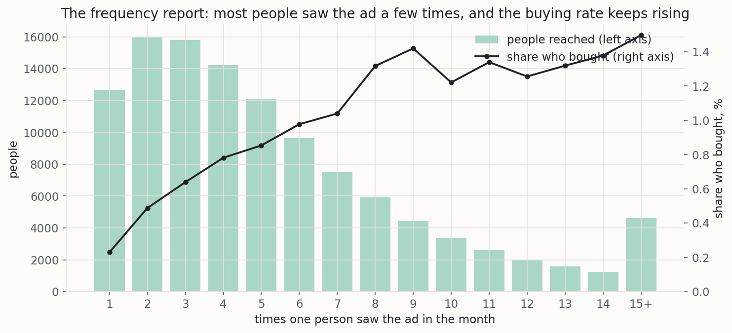
The intuition. Picture the frequency report as a row of buckets: everyone who saw the ad once, everyone who saw it twice, and so on up to fifteen or more. Draw the share who bought in each bucket and you get a line that rises and flattens. The cap is not where it goes flat. It never quite does. The cap is where the rise from one bucket to the next stops being worth an impression.
Put prices on it. Say an impression costs 1.2 cents and a sale is worth 25 euros.
Then one more impression pays only while it lifts the chance of a sale by more than 1.2 in 2,500, about one extra buyer for every two thousand people shown it. Past that, I am buying impressions that cost more than they return, and the platform will sell me as many as I like.
Now picture the audience as a race most entrants never finish. Everyone starts the clock when they join. The buyers cross the line at different times and the never-buyers run forever. The half-life is the time by which half of the finishers have finished. How stale an audience is depends on how much of its buying is still to come, which is a question about the finishers only.
The formula, written out
Here is all the maths. It takes five lines, and every number later in the post comes out of them.
The saturation curve is the Hill curve, three numbers describing a rise that flattens:
CVR(f) = CVRmax · fn ÷ (Kn + fn)
- f is how many times a person has seen the ad.
- CVRmax is the ceiling, the share who would buy if the ad could be shown without limit.
- K is the half-way point, the frequency at which the share reaches half the ceiling.
- n is the shape. Below one, the first impression does the most. Above one, the first impression or two do little and the curve speeds up before it flattens, the S-shape the effective-frequency school described when it concluded that a single exposure within a purchase cycle usually does little or nothing [2]. The fit chooses the shape.
I fit the curve by least squares, weighting each bucket by the people in it, so a thin bucket cannot drag it about. Two checks stand in front of any cap. The curve must beat a flat line by more than chance would, because a fit always returns numbers, even on an audience whose buying does not move with frequency. And the cap must sit inside the frequencies the audience reached.
The cap is where the next impression stops paying. The slope of the curve is how much one more impression adds to the chance of a sale:
dCVR ÷ df = CVRmax · n · Kn · fn−1 ÷ (Kn + fn)2
An impression pays while that slope, times what a sale is worth, beats what the impression costs. Divide through by the value of a sale and the cap is the last frequency where the slope still clears
τ = cost of one impression ÷ value of one sale
a number you own, not one the curve owns. The notebook reads it as the whole number of impressions that makes a reached person worth the most: the value of a sale times the curve, minus the cost of an impression times the frequency.
The audience's decay is a survival curve with a never-buyer share. The share of the audience that has not bought by age t is
S(t) = (1 − c) + c · exp[ −(t ÷ λ)k ]
- c is the share who will ever buy. The curve flattens at 1 − c, the never-buyers, instead of falling to zero.
- λ (the scale) and k (the shape) describe when the buyers buy. This is the Weibull, the one simple family that can say a buyer who has waited is getting more likely to buy, less likely, or neither [3].
The three numbers are chosen to make the data most likely. A person still unbought counts as not having bought yet, either a never-buyer or a buyer whose time has not come, and that is the part the rate-by-age table throws away. It is the problem Kaplan and Meier's estimator was built for: an event you were waiting to see, hidden because something else happened first [4].
The half-life is the age by which half of the eventual buyers have bought. It is the middle of the buyers' curve, not the whole audience's, which never reaches one half when most people never buy:
H = λ · (ln 2)1 ÷ k
The worked example synthetic
The audience. One online store's retargeting audience, shown the ad for twenty-eight days (synthetic, built so the right answer is known in advance). The ad reached 113,591 people and 943 of them bought.
Each person's built-in curve starts slowly, rises and flattens. I also built in a lean, because real delivery has one: the platform sends more impressions to keener people, so the people who saw the ad twelve times were 1.24 times as keen as those who saw it twice. The lean is the one number in this notebook that is assumed rather than measured, because in a real account it is exactly what a report cannot show.
| the audience | value |
|---|---|
| people reached over twenty-eight days | 113,591 |
| share who bought | 0.83 per cent |
| times the median person saw the ad | 4 |
| mean times seen | 5.5 |
| one in ten saw it at least | 11 times |
| an impression costs | 1.2 cents, €12 per thousand |
| a sale is worth | €25 of margin |
| an impression pays while it lifts the chance of a sale by more than | 0.048 per cent of people |
The report. The share who bought rises overall, dips here and there, and is highest in the top row, never settling into a peak. So cap where the rate stops improving says no cap at all. Three a week says twelve.
| times seen | share who bought |
|---|---|
| once | 0.23% |
| twice | 0.49% |
| three times | 0.64% |
| five times | 0.85% |
| eight times | 1.32% |
| fifteen or more | 1.50% |
The fit. The curve beats a flat line by far more than chance would: the chance of a fluke is smaller than one in a billion billion billion billion. Nobody has ever been that sure about my retargeting. At these prices the fitted curve puts the cap at 10 impressions a month, inside the frequencies the audience reached.
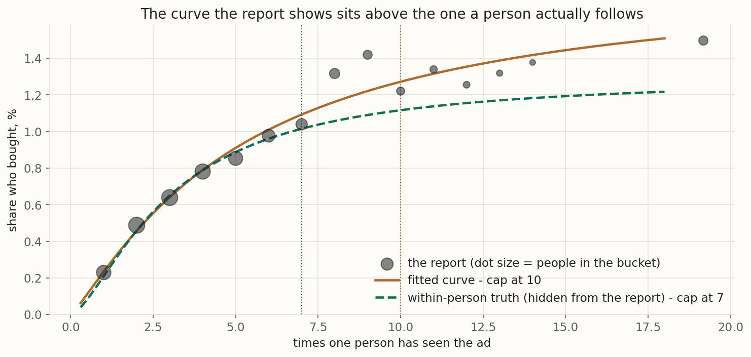
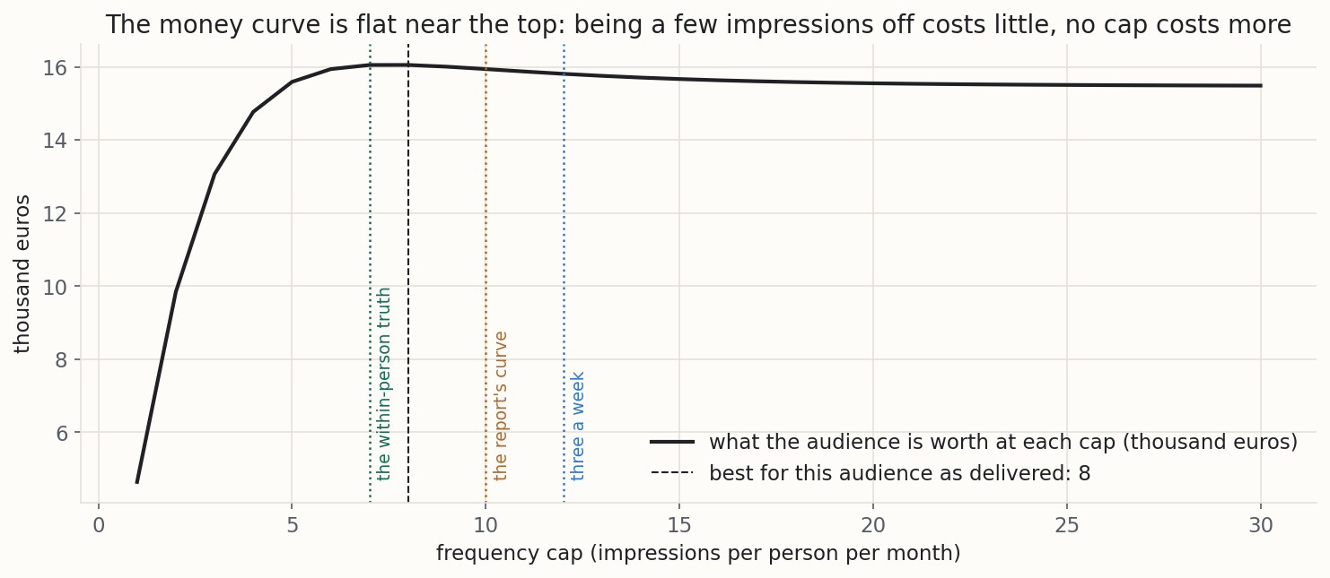
What the report cannot see. The curve I built in, at the same prices, caps at 7. The report's curve sits above it past three impressions, because the heavy buckets hold keener people, so the cap it reads is three impressions late. A subtlety runs the other way: capping the heavy viewers costs more than the average person's curve says, because they are the keener ones. So the cap that is actually best for this audience as delivered is 8, between the two.
| ceiling | half-way point | shape | share at ten impressions | |
|---|---|---|---|---|
| the truth I built in | 1.3% | 3 impressions | 1.5 | 1.12% |
| the curve fitted to the report | 1.85% | 5.2 impressions | 1.18 | 1.27% |
What that is worth. This audience costs €7,432 a month to serve with no cap. No cap at all leaves about 7.8 per cent of the audience's spend on the table.
The three-a-week rule of thumb lands at 12 and costs about 3.3 per cent of the spend. Being two or three impressions off costs little. Having no cap costs most, because I pay for the people who saw the ad twenty and thirty times.
| cap | left on the table each month | share of the uncapped spend |
|---|---|---|
| 8, the best for this audience | nothing | nothing |
| 10, the report's cap | €113 | 1.5% |
| 12, three a week | €243 | 3.3% |
| no cap | €579 | 7.8% |
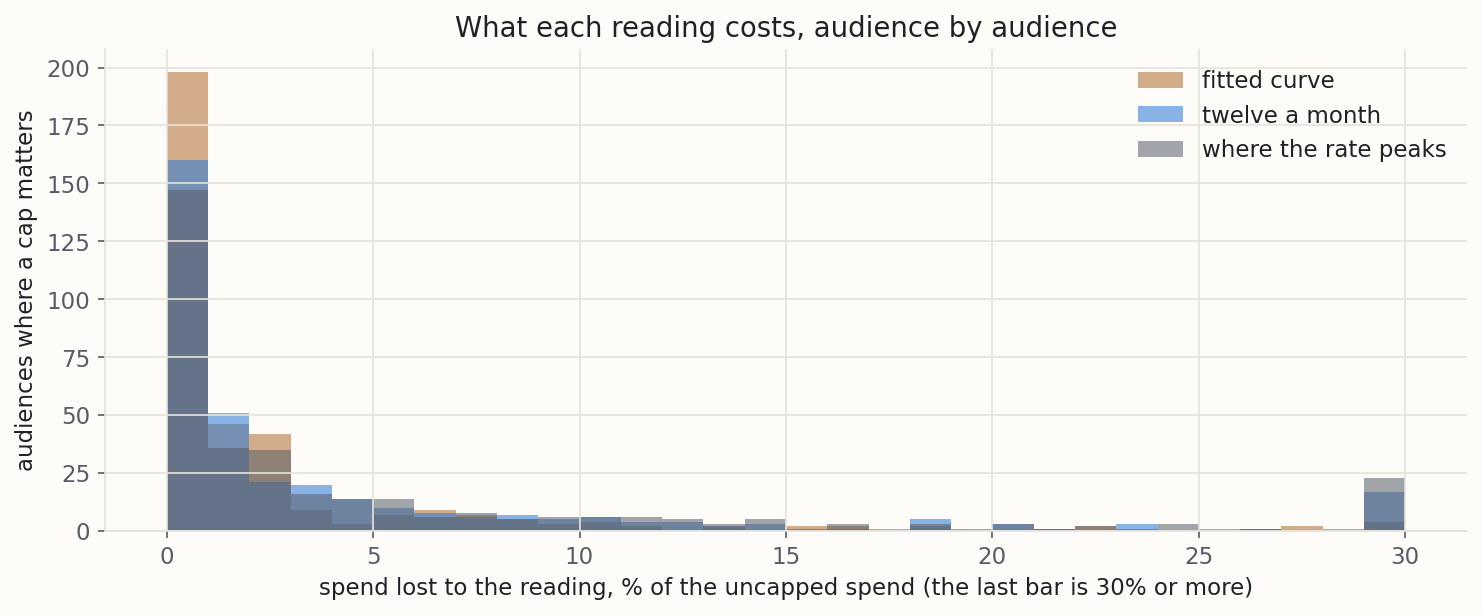
Scored on five hundred audiences. One audience proves nothing, so the notebook builds five hundred (499 had enough data to score), each with its own curve, size, prices and lean. On 71 per cent of them the best cap sits inside the frequencies reached, so a cap matters. On the rest the right answer is no cap. Here is what each reading leaves on the table, as a share of the uncapped spend:
| reading | typical audience | worst tenth | imposes a cap where none is needed |
|---|---|---|---|
| the fitted curve | 0.4 % | 7.5 % | 29 % of the time, costing 0.1 % |
| the fitted curve, unweighted | 0.7 % | 9.8 % | 32 %, costing 0.2 % |
| where the rate peaks | 2.0 % | 19.0 % | 68 %, costing 2.6 % |
| twelve a month | 2.9 % | 20.7 % | 100 %, costing 8.9 % |
| no cap | 1.4 % | 16.2 % | never |
Where the best cap sits decides whether twelve was a good guess. On audiences whose best cap is nine to fourteen, the rule narrowly beats the curve. Where it is under five, the rule loses about a quarter of the spend and the curve loses nothing. A rule of thumb is right when it happens to be right.
| where the best cap sits | twelve a month loses | the fitted curve loses |
|---|---|---|
| under five | 23% | none |
| nine to fourteen | 0.2% | 0.8% |
| fifteen to twenty-four | 1.7% | 0.5% |
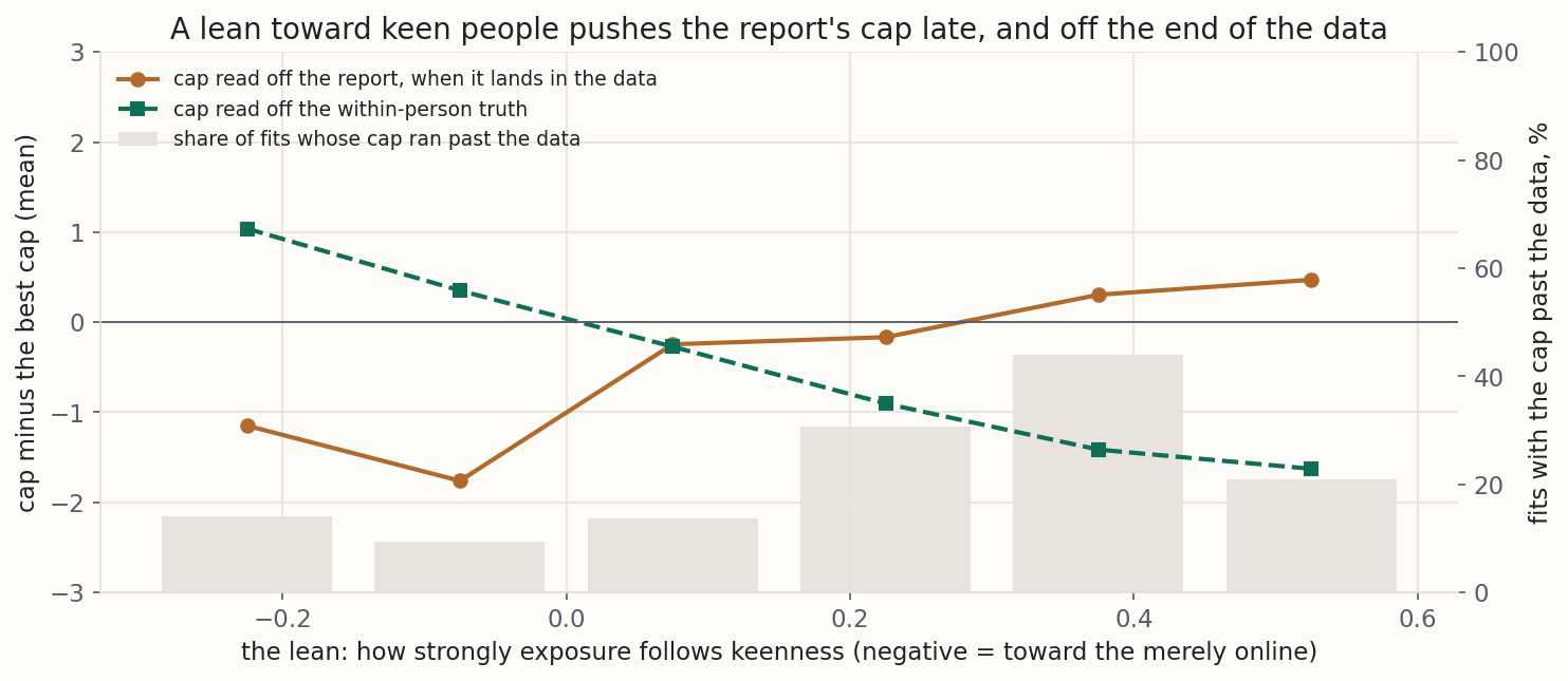
The lean, measured. A lean toward people who are merely online more pulls the report's cap about an impression early. A strong lean toward keen people pushes it late, by under half an impression, and more visibly off the end of the data; a moderate one leaves it on time or a little early. The report cannot tell you which way its lean runs. That is what a holdout is for.
The gate, measured. On five hundred audiences whose buying does not move with frequency at all, the fit hands back a cap on 100 per cent of them with the gate off and 1.8 per cent with it on. On the audiences that do bend, the gate refused 3.8 per cent, which is its price.
The fitted cap sat beyond the top bucket on 35 per cent of all audiences, and on 71 per cent of those where no cap was right. That is the method saying so in the only way it can.
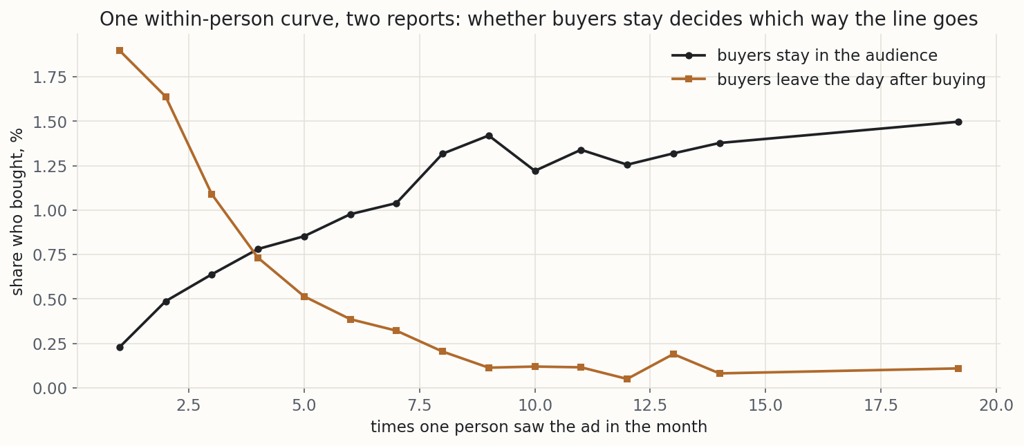
When buyers leave the audience. Most retargeting audiences drop people once they buy. Run the same audience that way and the report turns upside down: the share who bought falls from 1.90 per cent among people who saw the ad once to 0.11 in the fifteen-or-more bucket. A person who buys at their fourth impression stops at four, while a person who never buys keeps going to twenty.
Cap where the rate peaks now says cap at 1. The fitted curve finds nothing that bends upward at all. Neither is the answer, because in that report frequency is partly a result of buying rather than a cause of it, and the notebook's loader warns when a report has that shape.
The half-life. The same store's audience, watched for sixty days: 20,000 people joined and 1,971 had bought by the end. In the truth I built in, 12 per cent will ever buy, and half of them have bought by day 9.2.
The rate-by-age table makes the audience look twice as patient as it is. A Weibull with no place for never-buyers explains them as buyers who take more than a year. My method reads 9.4 days and a 12.0 per cent ever-buy share.
| reading | half-life |
|---|---|
| the truth I built in | 9.2 days |
| the rate-by-age table | about day 20 |
| a Weibull on the buyers alone | 8.3 days |
| a Weibull with no place for never-buyers | 449 days |
| my method | 9.4 days |
| half-lives since joining | share of the eventual buyers who have bought |
|---|---|
| two | 84% |
| three | 96% |
| four | 99% |
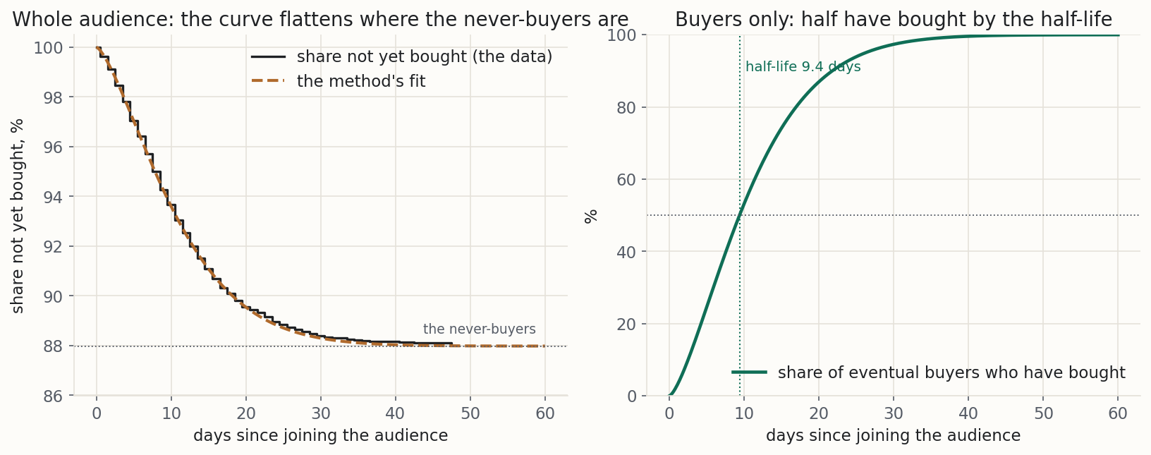
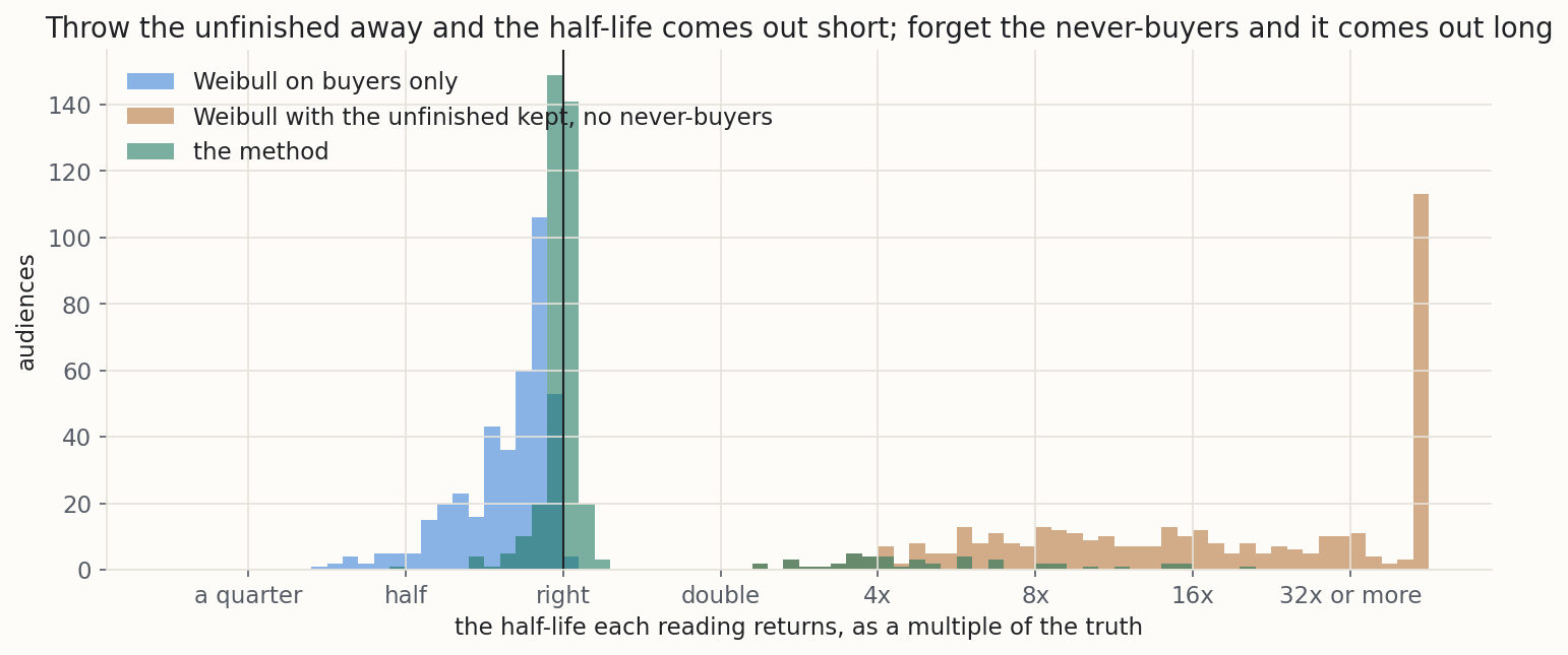
On four hundred audiences, my method came out right on the typical audience and within twenty per cent of the truth on six in seven. The seventh it misses is the one watched too briefly.
| reading | typical half-life against the truth | within twenty per cent of the truth |
|---|---|---|
| the rate-by-age table | 1.8 times | 12% of audiences |
| buyers alone | 0.84 times | 58% |
| no place for never-buyers | 17 times | never |
| my method | 1.00 times | 86% |
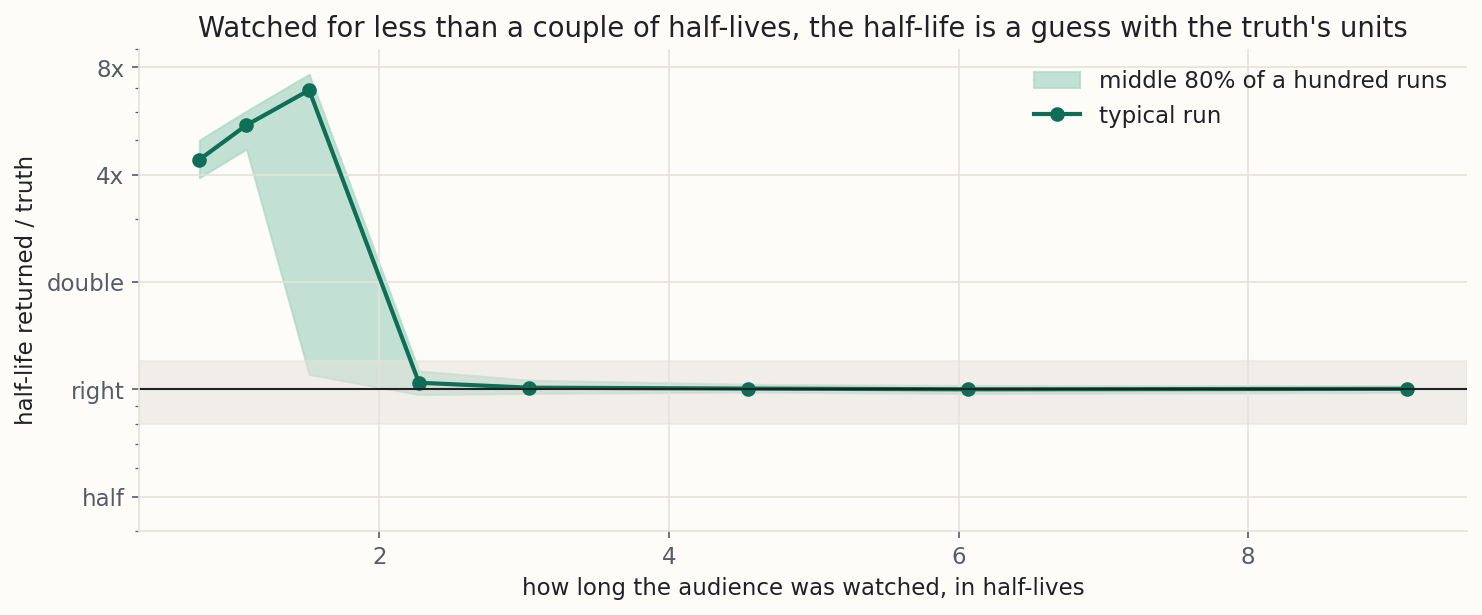
How long you have to watch. The never-buyer share can only be told from slow buyers once the curve has had time to flatten. Watched for one week, the method's half-life comes out at over four times the truth. At a fortnight it is right on one run in six. At three weeks, 97 per cent of runs land within twenty per cent, and from four weeks all of them do. In the audience's own units, that is three half-lives of history before the number can be trusted.
When two audiences hide in one. A three-day promotion brings 2,872 joins a day into an audience that normally takes 198, and its buyers are deal-seekers who buy fast or not at all.
The steady trickle's half-life is 9.6 days and the promotion's is 4.8. Read across the whole pool, the half-life comes out at 6.4 days, which belongs to neither group.
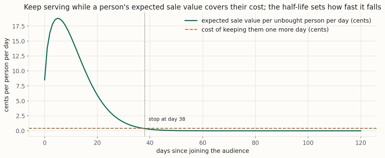
What the half-life is worth. Keeping one person in the audience costs about 0.42 cents a day. An unbought person's expected sale value tomorrow falls as they age, and it falls under that cost at day 38, about four half-lives.
That assumes every sale an audience member makes is the ads' doing, the strongest assumption available. If only half are, the window shortens to 34 days, and if a quarter, to 30. The default of thirty is not far off here. Ninety is.
| keep people for | left on the table against the best window |
|---|---|
| thirty days | €627 |
| sixty days | €1,257 |
| ninety days | €3,470 |
| a hundred and eighty days | €10,121 |
Try it on your own numbers
Pick one of four synthetic frequency reports, set what an impression costs you and what a sale is worth, and watch the fit, the gate and the cap move. Below it, move the share who will ever buy and the buyers' timing, and read the half-life and the membership window. The pinned cases are the ones the notebook stores, and the widget reproduces all of them with the same maths and says so at the bottom.
Caveats: where the two curves lie to you
Every method has conditions it needs, and these are the conditions my two curves need. They are the part of the post worth reading twice.
The report's curve is not the person's curve, and it cannot tell you which way it is off.
If the platform sent the heavy doses strongly to keen people, the report's cap runs late, often past the end of the data. If it sent them to people who are simply online more, the cap runs early. The report cannot show which, and only a holdout sees it.
A cap belongs with its window.
The effective-frequency review scoped every conclusion to a single purchase cycle [2], because the mechanism underneath is forgetting. A cap of twelve in twenty-eight days is not a cap of three in seven, so compare this curve only with caps over the same twenty-eight days. My synthetic audience never forgets, so the notebook cannot measure how much the window matters. Real people do forget.
A retargeting audience restarts its clock on every visit.
Most platforms reset membership each time a member comes back, so the join date in the export is the latest qualifying visit, not the first. Counted from the first visit, a returning visitor looks older than the platform treats them. Counted from the latest, they look younger than they are. Use the starting point the platform uses for the window you are pricing, and say which.
A cap read past the top bucket is the shape guessing.
The paper this curve comes from warns that two such curves can be "nearly identical within that range, but diverge outside it" [1]. A cap beyond the frequencies the audience reached is the shape talking, not the data. It happened on about a third of my audiences, mostly where no cap was needed. The honest reading is at least the top bucket.
An S-shaped curve has a floor as well as a cap.
On an S-shaped curve the slope clears the cost of an impression twice: on the way up, where extra impressions start to pay, and on the way down, where the cap sits. Below the lower point an audience is paying for exposures that barely help. On the worked audience that point sits below one impression.
How sharply the curve bends carries the brand, not just the audience.
The effective-frequency review found that very large, dominant brands respond to repetition quite differently from average ones, because as a brand nears saturation its response curve bends sooner [2]. The fitted shape cannot separate the brand's place in its market from the audience's response. There is no test for this in the data. It is a fact the advertiser knows about themselves.
If buyers leave the audience, the report is not about saturation.
The same curve for each person produces a rising report when buyers stay and a falling one when they leave. A falling report tells you who bought early, not what repetition does. Read no cap from it.
A join-time burst mixes two audiences.
A promotion, a list import or a campaign can land a surge of joins in a few days. Those people behave as a group, and the half-life of the mixed pool describes neither them nor the steady trickle. Fit the burst separately once it has enough buyers, or read the half-life off the quiet weeks.
Watched too briefly, the half-life is a guess with the truth's units.
Below three half-lives of history the never-buyer share is not pinned down, and the fit returns a number anyway. The notebook flags it. A week-old audience returned a half-life of forty-four days against a truth of nine.
Both numbers cap at "modelled".
Neither curve saw an experiment. Both describe the audience as it was delivered and when it bought, not what the ads did. Where a cap or a refresh matters enough to pay for a holdout, I would run one. Until then these are the best available answers, not measured ones.
These numbers are from synthetic data.
The audience, its lean, its buyers and their timing are what my generator produced, with the answers built in so every reading could be scored against a known truth. Yours has a different shape. The method travels and the numbers do not, which is why the notebook reads the cap and the half-life off your files.
Getting your data
The frequency report is one line per frequency bucket, three columns, in any order:
| column | what it holds | example |
|---|---|---|
frequency | times a person saw the ad in the window, and the top bucket may be written 15+ | 3 |
reach | people in that bucket | 16240 |
conversions | of those people, how many converted | 271 |
Here is the awkward part. The standard dashboards do not give you this. Meta's frequency breakdown counts people at each frequency, not conversions, and only for reservation buying [7]. Google Ads' frequency distribution counts people too, in cumulative buckets from one-plus to ten-plus [8].
The curve needs conversions by frequency, which only a per-person log of impressions and conversions can give. Campaign Manager 360's Data Transfer files are such a log, though the identifier can be zeroed out for privacy, and then the join cannot be made [9]. Email and push tools are the cleanest case, because they know how many times they sent to each person and who bought. The notebook's consolidator turns the two logs into buckets.
The audience file is one line per person, three columns:
| column | what it holds | example |
|---|---|---|
joined | the date the person entered the audience | 2026-05-03 |
converted_on | the date they bought, or blank if they have not | 2026-05-11 |
as_of | the date the export was taken, the same on every line | 2026-07-01 |
From a raw events log, such as a GA4 export or a CRM's activity table, the notebook takes the first visit as the join and the first purchase after it as the conversion.
What it refuses. A report with fewer than four frequency buckets holding people, or fewer than 50 conversions, which is where my measurement says the worst tenth of audiences start losing more than a tenth of their spend to a fitted cap. An audience file with fewer than twenty buyers. It warns, rather than refuses, when the cap lands past the top bucket, when the share who bought falls with frequency, and when the audience has been watched for fewer than three of its own half-lives.
The notebook runs on your own computer. Nothing about your account leaves it.
The same numbers, in production
The two platforms that sell most of the world's retargeting both treat a frequency setting as a count over a period, never a bare number. On Meta's reservation buying, a cap is a count within a reset period, for example no more than 3 times every 48 hours, enforced over a rolling window [10]. Google's YouTube product sells the frequency itself, as Target frequency, and its help page says plainly: "No, this is not a frequency cap." [11] Both are the window caveat, written into the product.
The audience half of this post replaces a default. Google's data segments keep members for thirty days unless you choose otherwise, up to five hundred and forty, and the help page advises choosing by how long the ads stay relevant to your visitors [12]. The half-life answers that with a number.
Common questions
What frequency cap should I set?
My frequency report shows the conversion rate falling as frequency rises. Should I cap low?
Is three a week right?
Does the cap change if my CPM changes?
How long should my retargeting window be?
My audience is a week old. Can I read its half-life yet?
Should I just run a holdout?
Run it on your own audience
Export one retargeting campaign's impressions and conversions per person for the last twenty-eight days, and its audience's join and purchase dates. Give both files to the notebook with what you pay per thousand impressions and what a sale is worth, and read the cap and the half-life it hands back. The spreadsheet carries the same fit, gate and cap in live formulas. Both run on your own computer and neither uploads anything.
In my synthetic store, half of the eventual buyers had bought within 9.4 days of joining, and keeping people stops paying at about 38 days. Yours will differ. Next Wednesday, when someone at the end of the table asks to show it more and keep people for ninety days, you can tell them where the next impression stops paying and what the extra sixty days cost.
References
- [1] Jin, Y., Wang, Y., Sun, Y., Chan, D. and Koehler, J. (2017). Bayesian Methods for Media Mix Modeling with Carryover and Shape Effects. Google Inc., pages 3 and 5.
- [2] Naples, M. J. (1979). Effective Frequency: The Relationship Between Frequency and Advertising Effectiveness. Association of National Advertisers, printed pages 63, 64, 67, 72, 73 and 77.
- [3] Helsen, K. and Schmittlein, D. C. (1993). Analyzing Duration Times in Marketing: Evidence for the Effectiveness of Hazard Rate Models. Marketing Science, 12(4), 395 to 414, pages 398 and 399.
- [4] Kaplan, E. L. and Meier, P. (1958). Nonparametric Estimation from Incomplete Observations. Journal of the American Statistical Association, 53(282), 457 to 481, page 457.
- [5] Fader, P. S., Hardie, B. G. S. and Lee, K. L. (2005). "Counting Your Customers" the Easy Way: An Alternative to the Pareto/NBD Model. Marketing Science, 24(2), 275 to 284, page 276.
- [6] McCarthy, D. M., Fader, P. S. and Hardie, B. G. S. (2017). Valuing Subscription-Based Businesses Using Publicly Disclosed Customer Data. Journal of Marketing, 81(1), 17 to 35, page 15 of the manuscript.
- [7] Meta for Developers. Breakdowns. Marketing API Insights documentation. Accessed 14 September 2026.
- [8] Google Ads Help. About frequency distribution. Accessed 14 September 2026.
- [9] Google for Developers. Data Transfer v2.0, Campaign Manager 360: overview and file format. Accessed 14 September 2026.
- [10] Meta for Developers. Ad Account Reach and Frequency Prediction. Marketing API reference. Accessed 14 September 2026.
- [11] Google Ads Help. About Target frequency. Accessed 14 September 2026.
- [12] Google Ads Help. How your data segments work. Accessed 14 September 2026.
From Stochastic Strata. I build marketing measurement that shows its working: every number carries its range, and when the data cannot answer a question, I say so and tell you what would. The worked example here is synthetic. The method is the real thing, and you can run it on your own data with the notebook or spreadsheet above. Nothing in this post is financial advice.