Significance testing · 14 min read · Interactive · Video
Is this difference real, or am I looking at noise? A two-proportion test and the Benjamini-Hochberg correction
It is Monday morning and the weekly report is up on the big screen. Mobile converts at 2.4%. Desktop converts at 1.9%. Somebody says what the room is already thinking, that mobile is the better placement, and by lunch the budget has moved. Maybe that was right. But the gap on the screen is doing two jobs at once, and only one of them is about mobile. The other is about how many clicks sat behind each number, and how many other rows everyone scrolled past before this one caught the eye. I have moved budget on a gap like this myself, more than once. This post is about how to tell.
The short answer
Often you are looking at noise, and two checks tell you which. First, the gap has to be bigger than the clicks behind each number allow, which the two-proportion test from any statistics textbook checks from the raw counts rather than the percentages. Second, if you found the gap by scanning a breakdown table, you correct for every row you scanned, using the false discovery rate procedure that Benjamini and Hochberg published in 1995.
The scanning matters more than people expect. In my simulations of tables where every row converted at the same true rate, 86.0% of forty-row tables still showed at least one difference that was not there. Correcting for the scan cut the average account's share of wrong flags on realistic tables from 55.7% to 4.4%, inside the 5% it promises.
The correction cannot create evidence the counts do not hold. At everyday volumes it misses most of the real differences too.
Which methods this uses, and why not the others
Four plain tools do the work, and all of them run on counts you already have. A two-proportion test asks whether the gap between two rates is bigger than the clicks allow. A score interval, Wilson's from 1927 [1], says what a single rate could really be when a row has almost nothing in it. The false discovery rate procedure [2] accounts for having looked at forty rows instead of one. A separate ratio test handles cost per acquisition, which is not a rate and does not behave like one. Nothing is fitted or trained, and you can check every step by hand.
Three other tools are each better than mine at something, and none of them answers this question.
Machine learning. It finds patterns across many variables at once. It also wants thousands of conversions per segment, not dozens, and it predicts rather than weighs evidence. It will rank forty rows for you without ever saying whether any difference is real.
A Bayesian test. It copes well with tiny counts and answers the question a marketer actually asks ("what is the chance B beats A?"). For one planned comparison at low volume it is the stronger tool. The price is a starting belief, called a prior, that you must choose and defend, and its headline number reads as more certain than it is, which on a forty-row table makes scanning worse.
A real randomised split test. It settles cause, which nothing here can. But you cannot randomise somebody's device, region or match type. Those belong to the visitor, so for a breakdown table the gold standard does not apply. Where you can randomise, run the experiment instead.
I stay with the plain tests because they need only the counts every export already gives you, and a method you can check by hand is a method you can argue with.
The question underneath
Every job in this trade is comparisons. This week against last. This audience against that one. A breakdown table is a machine for producing them.
The hard part is not the arithmetic. A percentage hides the two things you need. A rate of 2.4% does not say whether it came from 50 clicks or 50,000, and the report does not say how many other percentages you looked at first. Strip both away and you are reading the shape of random variation and calling it a decision.
Why the reflex fails
The rule almost everyone runs is some version of it is more than a fifth off the average. On one comparison at decent volume it is not even bad. It fails on a table, because a table is mostly thin rows. Here is one account (synthetic, built so the right answer is known in advance): 40 segments, of which three genuinely convert at a different rate and thirty-seven do not.
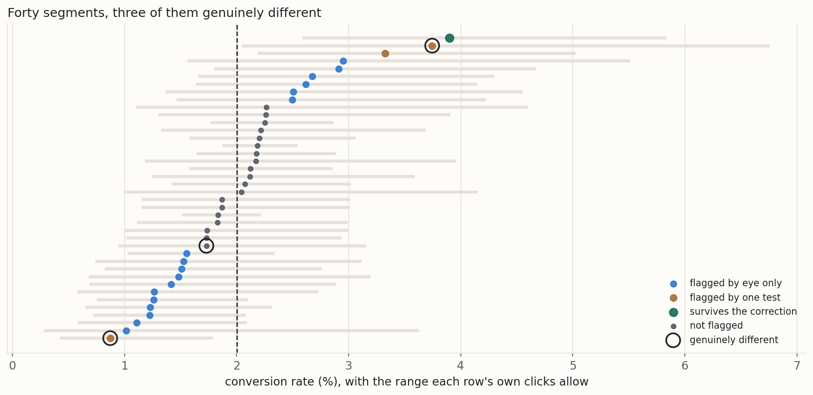
On the thin rows those ranges stretch across most of the chart. The reflex flags 21 of the forty rows. Most of the table looks noteworthy, which is another way of saying none of it does.
One account is one draw. In this one, a real difference was never flagged by anything, and the single row the correction kept was not one of the three. That is why every other number in this post is an average over 400 simulated accounts rather than a story about one.
The test, term by term
Here is the one stretch of maths. It is a single formula, and after it you can check the rest by hand.
z = (p̂a − p̂b) ÷ √( p̂ (1 − p̂) (1/na + 1/nb) )
where p̂ = (xa + xb) ÷ (na + nb)
- xa, na are the raw counts for the first group, conversions and clicks. Not the rate, which has already thrown away the number of clicks.
- p̂a is that group's rate, xa ÷ na.
- p̂ is the pooled rate, both groups added together as if they were one. You are testing whether the two are the same, so the noise is measured as if they were. Swapping in an unpooled version is the most common way this test is misused.
- The bottom of the fraction is how much the gap would wobble if nothing were going on. It shrinks as either group collects clicks, so the same gap alarms you on a heavy comparison and bores you on a thin one.
The result, z, is the gap in units of its own noise. It converts to a p-value, the probability of a gap at least this big if the two rates were really identical. Small p, hard to explain away.
Thin rows, and the range that lies about them
The other half of the problem is a row with almost nothing in it. A segment with a few dozen clicks and one conversion still produces a percentage, and a percentage looks like a number whether or not anything stands behind it.
The textbook range around a rate, the rate plus or minus a couple of standard errors, behaves badly exactly here. Three statisticians who studied it put it bluntly: "the chaotic coverage properties of the Wald interval are far more persistent than is appreciated" [3]. I wanted to see that on marketing-sized numbers, so the notebook measures it.
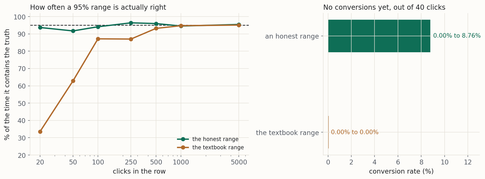
A range labelled 95% should contain the true rate 95 times in 100. At 20 clicks the textbook range manages a third of the time (33.5%), and it is still short at 250 clicks. The score interval this post uses instead [1], [4] stays close to its promise, though near a rate of zero it has known dips at every sample size [3].
The clearest case is a row where nothing has converted yet. Out of 40 clicks with no conversions, the textbook range runs from zero to zero, total certainty from no evidence. The honest range runs up to 8.76%. You have not yet ruled out a perfectly healthy rate.
| Clicks behind the rate | Textbook range contains the truth | Score range contains the truth |
|---|---|---|
| 20 | 33.5% | 93.7% |
| 50 | 62.8% | 91.7% |
| 40, no conversions | range 0.00% to 0.00% | range 0.00% to 8.76% |
The trap is the table, not the test
This is the part that matters most, and the part no dashboard does for you. A single test at the usual threshold is wrong one time in twenty when nothing is going on. That is the deal you sign when you pick the threshold, and on one comparison it is a good deal. It stops being a good deal when you make the comparison forty times. And you do, not on purpose, but by scanning.
To show it, I built accounts with no real differences at all, so every flag is false by construction. The only thing that changes across the chart is how many rows were looked at.
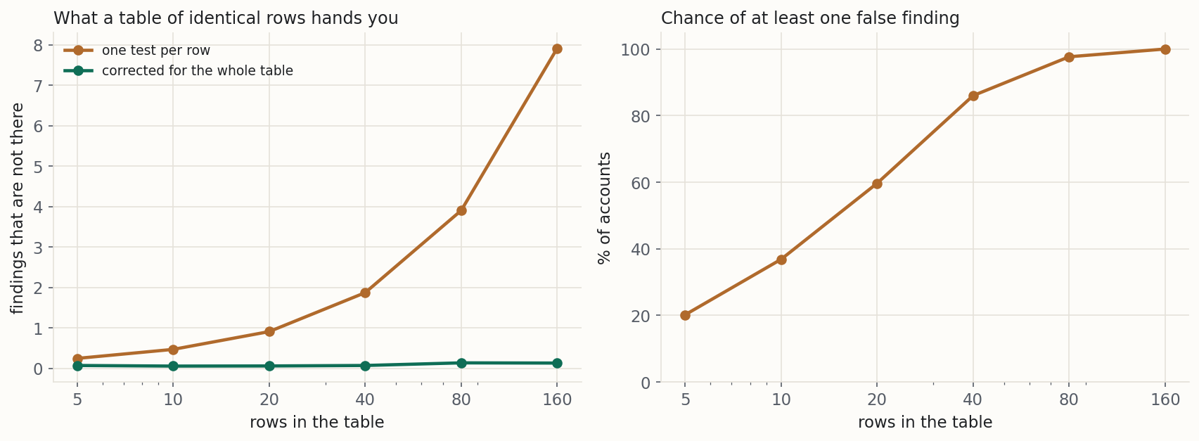
A device-by-region breakdown of a mid-sized account is easily eighty rows. On a table where nothing is happening, that hands you 3.90 findings on average, and nearly every account (97.7%) gets at least one.
The fix is Benjamini and Hochberg's, and it does not stop every mistake. It controls what the authors call "the expected proportion of errors among the rejected hypotheses, which we term the false discovery rate" [2, p. 290]. In marketing terms, that is the share of the rows you flagged that are wrong, the number you actually feel, because those are the rows you spend next week on.
rank the p-values smallest to largest, and the row at rank k out of m must clear (k ÷ m) × q
The smallest p-value faces the harshest bar and the largest the gentlest. It is arithmetic you can do in a spreadsheet, and the one below does it.
| Rows in the table | Findings that are not there | After correcting | Chance of at least one |
|---|---|---|---|
| 5 | 0.24 | 0.07 | 20.2% |
| 10 | 0.47 | 0.05 | 36.8% |
| 20 | 0.91 | 0.06 | 59.7% |
| 40 | 1.87 | 0.07 | 86.0% |
| 80 | 3.90 | 0.13 | 97.7% |
| 160 | 7.92 | 0.13 | 100.0% |
What correcting costs
It costs real findings, and a post that skipped this would be selling something.
I ran three readings over the same 400 realistic accounts, each hiding three real differences among its forty rows. The reflex flags 18.4 rows per account, and 87 flags in 100 are wrong. One proper test per row flags three, still mostly wrong. The corrected reading flags one row in every two accounts. Averaged account by account, which is what the correction promises to hold under 5%, 4.4% of its flags are wrong. Pooled over all 400 accounts the share is 12.7%, because the few accounts that flag anything flag only a row or two, so one wrong row weighs heavily.
Now the last column. The reflex finds 79.7% of the genuine differences, because it flags nearly half the table and catches things by sheer volume. The corrected reading finds 13.8%.
That is the right trade once you see what it says. At these volumes most real differences in a breakdown table cannot be found, and most of what looks findable is not real. Even one proper test per row, before any correction, finds only 41.4% of them. The clicks are simply not there.
So the best answer is not a formula. Decide what you are testing before you look. One planned comparison at decent volume needs no correction at all. The correction is the bill for a scan you have already done.
| Reading | Rows flagged per account | Share of those flags that are wrong | Share of the real differences found |
|---|---|---|---|
| The reflex, a fifth off the average | 18.4 | 87.0% | 79.7% |
| One proper test per row | 3.0 | 59.0% | 41.4% |
| Corrected for the whole table | 0.5 | 12.7% | 13.8% |
Ratios are a different sum
Cost per acquisition is not a rate. It is one total over another, and its uncertainty is set by the number of events behind it. Twenty conversions at ten euros each and twenty at a thousand euros carry the same uncertainty about the cost per conversion.
z = log(Ra ÷ Rb) ÷ √(1/ca + 1/cb)
where R = total ÷ total, and c = the number of events
This test has a limit worth knowing first, so the notebook measures it. Both bars below are pairs of segments whose true ratio is identical, so every flag is false.
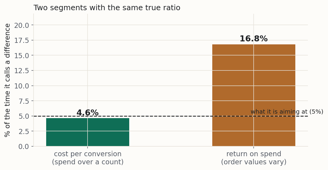
For cost per conversion, a spend divided by a count, the test cries wolf 4.6% of the time, which is what it aims at. For return on spend, where the top of the ratio adds up orders of different sizes, it cries wolf 16.8% of the time when order sizes vary as much as their average, more than three times its promise. The formula does not know about the spread between order sizes.
So this test is for cost-per-something. Point it at revenue-per-something and it will find differences that are not there, confidently.
A worked example
Two creatives in one campaign, at the volume where these decisions really get made (synthetic, with the answer known in advance, because on real data nobody knows which differences were real). Creative A converts at 2.42%, Creative B at 1.55%. A is converting more than half as much again as B. In a meeting, that is a decision: shift the budget, pause B, brief more like A.
Both rates came from exactly the same true rate of 2.15%. There is no difference between these creatives at all.
The test gives p = 0.28, so a gap this size turns up more than one time in four by chance alone. The honest ranges overlap across most of their length. You have not learnt which creative is better. You have learnt that twelve hundred clicks cannot tell you.
The gap on the screen was 0.87 points of conversion rate. Nothing about it was a lie. It simply was not evidence.
| Creative | Conversions | Clicks | Rate | Honest range |
|---|---|---|---|---|
| A | 15 | 620 | 2.42% | 1.47% to 3.95% |
| B | 9 | 580 | 1.55% | 0.82% to 2.92% |
Try it on your own numbers
Set the two rows' counts and watch the ranges move. Then move the last slider, how many rows you scanned before this one caught your eye, and watch the verdict change without a single count moving. That last control is the whole argument of this post, and no dashboard has it. The four presets are the cases the notebook pins. The widget reproduces all of them, and says so at the bottom.
Caveats to watch out for
Every method has conditions it needs. These are this one's, and they are the part of the post worth reading twice.
The correction assumes the tests do not lean on each other, and yours do.
Benjamini and Hochberg proved their 1995 result for independent tests. Rows of one account share traffic and seasons, and in the comparison used here each row shares a denominator with the group it is tested against. That ties the rows together in the opposite direction from the kind of dependence the 2001 companion paper proves safe [5]. Whether the guarantee survives is unproven, not shown wrong. The companion’s stricter version covers any dependence, at the cost of fewer findings. Treat the corrected count as a large improvement, not a proven guarantee.
Adding rows up mixes in what you added over.
Sum a breakdown across campaigns and each row carries its campaigns with it. If most remarketing traffic sits on computers, computers look better because of the campaign, not the device. Compare within one campaign, or check that the gap holds in each campaign before acting on the total.
Count each click once.
No row may have more conversions than clicks. A conversion action that counts every conversion, or weights by value, can report more, and fractional conversions from shared credit are modelled shares, not counts. Export one conversion per click. The notebook refuses a row that breaks this rule rather than testing it.
Real rows wobble more than coin flips.
The test assumes every click is an independent draw at one rate. Real segments drift from week to week beyond that. On a real store, a screen like this one flagged a row with no real difference 5.5 times as often as the label promises in a typical month. My platform measures that drift and discounts for it. On your own table, split the counts by week and check the gap holds in most weeks.
A p-value is not a probability that you are wrong.
It is the probability of a gap this large if there were no difference. How likely a difference is depends on how plausible it was before you looked. A p of 0.04 on a wild idea is much weaker evidence than a p of 0.04 on an expected one.
Not significant does not mean the same.
It means this data cannot tell them apart, which at marketing volumes is almost always the true statement. The worked example does not show the two creatives are equally good. It shows twelve hundred clicks is not enough to find out.
Significant does not mean worth acting on.
Pile up enough clicks and a trivial difference will clear any threshold. Read the size of the gap and its range beside the p-value, never the p-value alone.
The correction only covers the tests you tell it about.
Correct across forty rows, then go and look at a different breakdown, and you have started a new family of tests. The guarantee does not stretch across both. Decide the family before you look.
Your ad platform may call a row significant that this does not.
The platforms test one comparison at a time, at 95 per cent each, with no correction for testing several together. After the correction across the whole table, a row whose own p-value clears 0.05 can stay unflagged on purpose. It is held to a stricter standard, not hidden. If one row mattered to you before you looked, name it in advance and test it on its own.
A window that spans a change blends two rates.
A promotion, a tracking break or a new bid strategy part-way through the window means the early and the late clicks run at different rates, and the pooled rate describes neither. Cut the window at the change and compare the stretch after it.
Stopping when you like the answer breaks all of it.
Checking a test daily and calling it the moment it crosses the threshold produces false findings far more often than the label says. Everything here assumes you looked once, at a planned volume.
The ratio test is for cost-per-something.
Revenue-based ratios carry a second source of variation this arithmetic ignores, and ignoring it was measured: 16.8% false alarms against the 5% it advertises, more than three times its promise.
Getting your data
All of this runs on one table, one row per thing you want to compare.
| column | meaning | example |
|---|---|---|
segment | whatever you are comparing: device, region, creative, match type | mobile |
trials | the denominator: clicks, impressions, sessions | 4192 |
successes | the numerator: conversions, clicks, sign-ups | 88 |
Two rules matter more than they look.
Raw counts, never rates. If your export has a conversion-rate column, leave it out. The counts carry how much the number was allowed to move, and a rate has thrown them away.
Every row you looked at, not just the interesting ones. The correction needs to know how many rows you scanned. Hand it the three rows that caught your eye out of forty and it believes you ran three tests, so it will happily confirm all three. It is the easiest way I know to get a wrong answer out of a correct method.
The notebook reads your file from your own disk, and nothing is uploaded anywhere.
Common questions
What p-value should I use?
Is a bigger sample always the answer?
My A/B testing tool already reports significance. Is that not the same thing?
Can I just correct everything to be safe?
What if I only have a handful of conversions?
Should I not just run a proper A/B test instead?
Run it on your own table
Export last month's breakdown for one campaign, by device or by region, with clicks and conversions as raw counts and every row included. Run it through the notebook or the spreadsheet above and count how many rows survive the correction. Both run on your machine and neither uploads anything. Then, next Monday, when mobile beats desktop on the big screen, you can ask two questions before the budget moves: how many clicks, and how many rows?
References
- [1] Wilson, E. B. (1927). Probable inference, the law of succession, and statistical inference. Journal of the American Statistical Association, 22(158), 209 to 212. Accessed 8 September 2026.
- [2] Benjamini, Y. and Hochberg, Y. (1995). Controlling the false discovery rate: a practical and powerful approach to multiple testing. Journal of the Royal Statistical Society, Series B, 57(1), 289 to 300, p. 290. Accessed 8 September 2026.
- [3] Brown, L. D., Cai, T. T. and DasGupta, A. (2001). Interval estimation for a binomial proportion. Statistical Science, 16(2), 101 to 133, abstract, p. 101. Accessed 8 September 2026.
- [4] Agresti, A. and Coull, B. A. (1998). Approximate is better than "exact" for interval estimation of binomial proportions. The American Statistician, 52(2), 119 to 126. Accessed 8 September 2026.
- [5] Benjamini, Y. and Yekutieli, D. (2001). The control of the false discovery rate in multiple testing under dependency. Annals of Statistics, 29(4), 1165 to 1188. Accessed 8 September 2026.
From Stochastic Strata. I build marketing measurement that shows its working: every number carries its range, and when the data cannot answer a question, I say so and tell you what would. The worked example here is synthetic. The method is the real thing, and you can run it on your own data with the notebook or spreadsheet above. Nothing in this post is financial advice.