Interrupted time series · 13 min read · Interactive · Video

I changed something. Did it actually work? An interrupted time series

It is three weeks since somebody cut the target cost per lead, and the dashboard says cost per lead is up 4 euros. “Roll it back?” Not yet. On this account the change worked, and the average had it backwards.

Andrei PopescuMedia buyer passionate about measuring outcomes, and the writer of this blog.September 2026
Written against the cited papers

The short answer

You can tell, but not by comparing the weeks after your change with the weeks before. A metric that was already climbing keeps climbing, and that average hands you the climb as your result, sometimes with the direction backwards. The fair test projects the line your metric was already on past the change date and measures the gap. Statisticians call this an interrupted time series, and Google’s researchers built a close relative of it for advertising. Read the gap only for the few days the projection stays sharper than the metric’s own daily swing, and check that quiet dates do not fake an equally strong break.

In my synthetic tests three weeks of history was the floor; on the demo shop's real series, even four weeks claimed an effect that was not there 14 times in 100. With two, the range claimed an effect that was not there up to three times as often as it should. The method cannot see anything else that happened that week.

Watch · 11 min The whole method end to end: why the before-and-after average reverses the sign, what to compare against instead, the three checks that keep it honest, and where it stops.

Watch: the test that gets the direction backwards

Prefer to read? Everything below covers the same ground in more depth: the maths, a widget to play with, and the notebook and spreadsheet to run it yourself. The worked example is synthetic, and every number on screen is computed. (Narration is automated for now. Turn captions on with the CC button.)

Sources cited in the video: the wrong-sign finding from Baicker and Svoronos, 2019, the projection method and the difference between daily and whole-period ranges from Google’s CausalImpact paper (Brodersen and colleagues, 2015), and the placebo-test definition from Eggers and colleagues, 2024. The full list is in the references below.

The question this actually answers

Did the new bid strategy help? Did the bigger budget pay for itself? Did the new landing page do anything at all? The temptation is to compare the fortnight after with the fortnight before, and dashboards make it one click.

It fails for one reason. It assumes your metric was standing still, and almost none of them are. Costs drift up as auctions get busier, and conversion rates drift with the season. A metric that was already climbing keeps climbing after your change, and the average hands you that climb as if you had caused it. A metric that was already falling makes a change that did nothing look like a triumph.

The idea, in plain words

Stop comparing after with before. Compare after with what would have happened if nobody had touched anything.

Nobody can see that, but you can estimate it. The weeks before the change hold the pattern the metric was following: how fast it drifted, how much it bounced, how its Mondays differed from its Sundays. Fit that pattern, run it forward past the change date, and you have a line to measure against, which researchers call the counterfactual.

The gap between that line and what happened is your effect. The line is an estimate, so the gap comes with a range. That range is the honest part, and most before-and-after reports leave it out.

The formula, written out

Here is the maths in this post: two equations and a paragraph. You can skip to the worked example without losing the thread.

The pattern the model learns. It works on the daily change rather than the level, because levels drift and daily changes usually do not. Statisticians would call it a seasonal ARIMA model.

∇y_t = c + φ₁ ∇y_t−1 + Φ₁ ∇y_t−7 − φ₁Φ₁ ∇y_t−8 + ε_t

y_t: the metric on day t: cost per lead that day.
∇y_t: today minus yesterday: the daily move, which is what gets modelled.
c: a constant that sets the drift but is not the drift itself. The model projects c divided by (1−φ₁)(1−Φ₁): here about 54 cents a day, against the 9 cents a straight line shows (see the caveats).
φ₁: the weight on yesterday's move: whether a rise tends to carry on or partly reverse. Here it is about −0.1, a small reversal.
Φ₁: the weight on last week's move: the weekly shape, so this Monday's move resembles last Monday's.
φ₁Φ₁: the two weights together: a small correction, because the two weights multiply rather than add.
ε_t: the leftover: the genuine day-to-day randomness nothing explains.

Fit that on the days before your change, run it forward, and call each projected day ŷ_t.

The effect. Average the daily gaps across the days you are reading:

δ̂ = (1 / h) · Σ ( y_t − ŷ_t )

y_t: what actually happened on day t after the change.
ŷ_t: what the projection said would happen.
h: how many days you read (see below, it is fewer than you think).
δ̂: the average daily effect of your change.

The range needs care. Every day's projection leans on the same fitted pattern, so the daily errors move together, and averaging the single days' error bars quotes a range tighter than the data supports. Instead, draw a plausible set of the model's weights, simulate a whole path, record the gap, and repeat thousands of times. The spread of those gaps is the range. Brodersen and colleagues keep the same distinction, reporting pointwise intervals for each day apart from the effect over the whole period [1, p. 4].

A worked example synthetic data

The account below is synthetic, built so the right answer is known in advance, built by the notebook under one fixed seed. It is a lead-gen account: eight weeks of history, a cut to the target cost per lead, then three weeks of watching. Cost per lead was already drifting up by 17 cents a day, which a straight line through those eight weeks reads as about 9. Auction pressure, nothing dramatic.

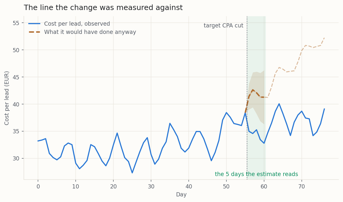
Cost per lead day by day: eight weeks of history drifting gently upward, a marked change date, then three weeks after it, with the projected line the post measures against. — Cost per lead before and after the change, with the projected line it is measured against.

What the before-and-after average says. Average the eight weeks before and the three weeks after, and cost per lead is up 4 euros, about 12 per cent. On that evidence you roll the change back.

What the projection says. Against the projected line, the same change made each lead about 7.50 euros cheaper a day, and the whole 95 per cent range sits below zero.

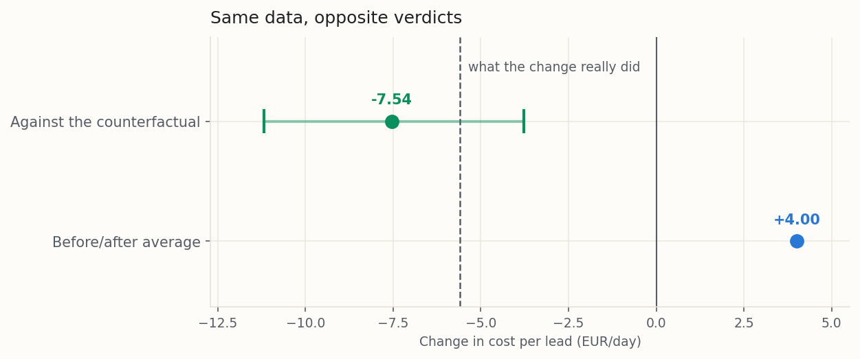
The before-and-after average and the counterfactual estimate side by side: the average sits above zero at four euros dearer, the projection sits well below zero with its range, and the built-in truth sits inside that range. — The before-and-after average and the counterfactual estimate, side by side.

I built the change to be worth 5.60 euros a day. The projection's range contains it. The before-and-after average does not merely miss it. It points the other way.

The estimate does overshoot, by nearly two euros. The projection overstates the weekly upswing that follows the change date, so the line it measures against sits about two euros too high across the five days I read. The range still contains the truth, which is what a range is for.

What I measured	Value
Days before the change, and their average cost per lead	56 days, €32.30
Days after the change, and their average cost per lead	21 days, €36.30
Before-and-after difference	€4.00 dearer, or 12.4%
Effect against the projection, per lead per day	€7.54 cheaper
95% range of that effect	€3.81 to €11.19 cheaper
Effect built into the account	€5.60 cheaper
Drift built in, read by a straight line, and projected by the model	17, 9 and 54 cents a day

How far ahead is it honest to look?

The projection gets vaguer every day it runs. Day one is a short step from data you saw. Day twenty is a guess built on nineteen earlier guesses.

At some point the projection becomes fuzzier than the metric's own ordinary swing from one day to the next, and past it every extra day averages in noise the projection invented. The range is tightest on the first day, so the window is a cap on how far you may read rather than a sweet spot. Read all of it, and no further.

The method finds that point from the data. On this account the metric's spread across the weeks before the change is 2.72 euros, and the projection's uncertainty passes it on the sixth day. So you read five.

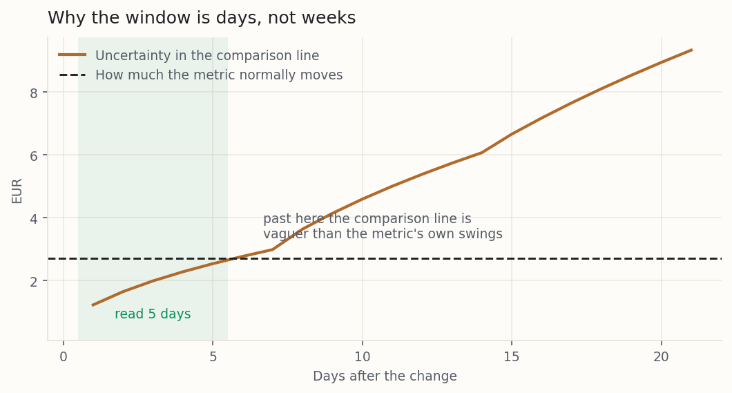
The projection's uncertainty growing day by day and crossing the metric's own normal daily swing on the sixth day, after five readable days. — The projection’s uncertainty growing past the metric’s own normal swing.

Five days. The before-and-after average happily used twenty-one, and every day past the fifth made its answer worse. This is the part that surprises people most: on a noisy metric, the reliable reading window is days, not weeks.

If five days feels too short to be useful, that is the honest signal, and the cure is a proper test next time. You can read longer, but the range widens faster than the extra days tighten it.

Could a quiet week have produced this?

Fair objection. This metric jumps about, so perhaps the model finds a break wherever you point it.

So point it somewhere nothing happened. Take dates from the quiet stretch before the change, pretend each was the change, and run the identical analysis. If they throw up breaks as strong as the real one, the analysis cannot tell your change from ordinary wobble.

Baicker and Svoronos suggest exactly this shape of check for a single series: try a break at every candidate date and keep the strongest score [2, p. 23]. Eggers and colleagues call it a placebo test, one that "checks for an association that should be absent if the research design is sound but not otherwise" [3, p. 6].

On this account seven quiet dates could be tested. The strongest of them scored 3.62. The real change scored 8.70.

Those scores are not euros. Each is the movement at that date divided by the noise around it, with the direction thrown away, because a quiet date can break either way. So the real change scored close to nine, while no quiet date managed even four. The noise in that score treats neighbouring days as independent, which they are not, so read it as a ranking of dates rather than a size. The score ranks dates rather than stating confidence, and the same formula scores every date, which is what makes the comparison fair.

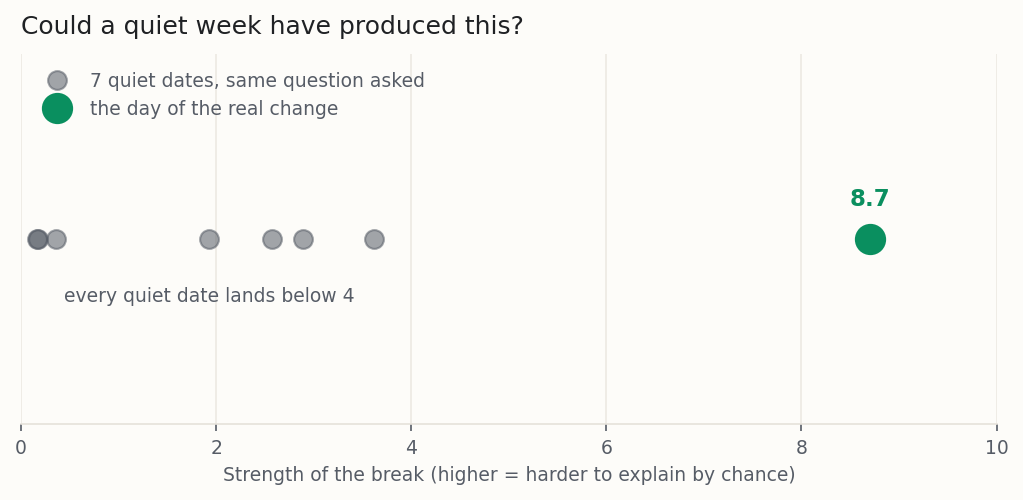
Seven quiet placebo dates scoring low on a break-strength axis, and the real change scoring far clear of all of them. — Seven quiet dates against the real change.

That gap is what turns "the model found something" into "the model found something your change caused."

Interactive Drag the reading window and watch the effect and its range move with it. It recomputes the article’s own quantity, the average gap between what happened and the projected line, so it opens on exactly the numbers above. Nothing leaves the page.

Play with the window

Caveats to watch out for in this method

This method earns a stronger claim than a before-and-after average. It does not earn certainty, and here is where it stops.

Something else happened at the same time.

This is the big one, and there is no clever fix. If a competitor entered your auction that week, or the platform changed its bidding, or demand moved, your number blends all of it together, and nothing in your own data can pull the strands apart. The method assumes your change was the only thing that happened, and that assumption is often false. How bad can it get? Baicker and Svoronos ran a single interrupted series on a randomised health experiment, where the true answer was known, and report that it "would have produced large and statistically significant results of the wrong sign" [2, p. 2]. Confidently backwards, with a tight-looking range around it. That is why the placebo test is not optional.

Your "before" has to be one world.

The projection assumes the weeks before your change were one stable stretch. If you switched bid strategy a month earlier, ran a promotion or broke a tracking tag, the model fits a blend of two worlds and projects a line that never existed. Check your change history and start the window after the last thing that happened.

Gaps break it outright.

The weekly part of the model counts rows, not dates, so across a missing day "the same weekday last week" is no longer seven rows back. A paused day makes such a hole, and so does a day with no conversions, where cost per conversion does not exist. The notebook spots this and falls back to the plain comparison, which is genuinely the weaker answer.

It only knows your weekly rhythm, never the year.

The model learns that this Monday resembles last Monday, and with eight weeks of history it could not learn a yearly cycle even in principle. A gentle seasonal slope gets absorbed into the drift, which is fine. A seasonal turning point near your change date is not. Demand recovers on its own, and the method hands you the recovery as your result.

The drift is the least pinned-down part of the fit.

On eight weeks of a wandering metric, the pace of the drift is hard to pin down, and neighbouring choices of model project the same weeks at paces several times apart. On this account the model projects about 54 cents a day where a straight line shows 9. The reading window is the guard, and it is the deeper reason the honest window is days, not weeks.

The range can be approximate.

If the leftover noise is lopsided, as it often is on cost metrics with their long expensive tail, the range is approximate: it may hold the true effect less often than 95 times in 100. If the pattern cannot be pinned down at all, the range loses its warrant. The notebook reports both conditions.

Short history can mean a falsely confident answer.

Three weeks of history is about where the weekly pattern becomes estimable at all. A 95 per cent range should claim an effect that is not there about one time in twenty. On test series with no effect and two weeks of history, mine did so up to three times as often. On the demo shop’s real series four weeks still did so 14 times in 100. The notebook warns below three weeks and refuses below two.

Changing because of a bad week flatters the change.

If you acted because the metric had just had a bad week, part of what follows may be the metric recovering on its own, and the model counts that recovery as your effect. Read the effect as possibly overstated. Comparing against other campaigns helps only if they dipped too.

A bid-strategy change has a learning period.

Google says a new or changed automated bid strategy spends a learning period recalibrating, and the first days are often the noisiest. A window of a few days can land inside it. Say so when you report the number, or read the window that starts once the strategy has finished learning.

It never proves causation.

Even a clean fit that passes every check is a modelled answer, because the comparison line was projected, never seen. Only an experiment sees it: hold your change back from a randomly chosen slice of the account and compare. When you can run one, run one. A geo-holdout is the natural partner, and this method is the honest second best.

Who actually uses this

Two public cases, and only two, because this section carries what can be sourced.

Google built a version of this for advertising measurement and released it. The paper behind its CausalImpact package demonstrates the method on the effect of an online advertising campaign on visits from search, and is candid that it is for "those settings where a randomised experiment is unavailable" [1, p. 1]. Their approach is Bayesian and mine is not, but the shape is the same: project the counterfactual, measure the gap, quote the uncertainty.

Health economists tested it against a known answer, and it failed. The Baicker and Svoronos study from the caveats is the most useful thing published about this method, because it is not a success story. They knew the true effect from a randomised experiment and ran the single-series version anyway [2, p. 2]. Read it before you lean on one of these numbers in a room where somebody is about to spend money.

Run it on your own data

Every download runs entirely on your machine, and your data never leaves it. They take one daily export: one row per day, covering a good stretch before your change.

column	meaning	example
`date`	a calendar date, one row per day, no gaps	`2026-03-02`
`cost`	what you spent that day	`412.55`
`conversions`	how many you got	`13`
`metric` (optional)	the number you want analysed, if you already have it	`31.73`

The notebook works out cost per conversion for you. If you already have the number you want analysed, put it in a column called metric instead. The notebook refuses to give a confident answer it cannot support. Too little history and it says so. A gap in the days and it falls back to the plain comparison rather than fitting something weaker in silence. A fit that fails its own checks and it tells you which one.

Notebook · PythonThe full method, executableFits the pattern on your pre-change days, projects it forward, reads the effect with its range, computes your own reading window from the data, runs the placebo test against quiet dates, and regenerates every figure here. Warns in plain words when the history is too thin or the checks fail.Spreadsheet · ExcelThe comparison, in live formulasA simplified workbook: the article's worked example as live formulas, and a your-data sheet you paste daily rows into, which projects the pre-change line forward and reads the gap. It flags in plain words when there are too few rows to trust the result.PDF · for your AIGive it to your assistantA brief to hand to ChatGPT or Claude. It walks you through exporting your daily cost and conversions, mapping the columns and running the notebook, one step at a time, with every caveat stated up front. No code experience needed.

Getting your data out of the platform

In Google Ads, pick the campaign, then Reports, Predefined, Time, Day, with Cost and Conversions as columns and no other breakdown. In Meta Ads Manager, use Ads Reporting and export with a Day breakdown, Amount spent and Results. If your conversions live in GA4, the notebook carries a BigQuery query for daily conversion counts, which you join to the ad platform's daily cost.

Two things people get wrong. If your export is split by campaign or device, total it per day first (the notebook has a helper). And the change date is the day the change went live, not the day somebody asked for it.

This part touches a spreadsheet or a light script, but you do not have to do it alone. Download the give-it-to-your-AI brief and hand it to ChatGPT, Claude or any capable assistant. It carries everything the assistant needs to pull your data, shape it and run the notebook, one step at a time, even if you have never written a line of code.

Common questions

How much history do I need before the change?

Eight weeks is comfortable. Three weeks is about the floor, and below that the answer can look more certain than the data behind it. More history helps until it reaches back into a period when something else changed.

How long should I wait after the change before measuring?

Less than you think, and the method works it out. On the account in this post it was five days, and waiting three weeks made the answer worse. On a metric built from conversions, also wait until those days have finished reporting, because conversions arrive late.

My before-and-after and this method disagree. Which do I believe?

This one, if your metric was moving before the change, which is the usual case and the reason they disagree. On a genuinely flat metric the two answers converge.

Can I use this on conversion rate, ROAS, or impression share instead of CPA?

Yes, any daily metric. Ratios with small denominators are noisier, so expect a wider range on a low-volume campaign. Impression share often sits steady rather than drifting, which the method detects and handles.

What if I made three changes the same day?

Then you measure the three together and cannot separate them. The honest report is "these changes together moved cost per lead by X." To know which one did it, change one thing at a time, or run a test.

Can I just run this continuously, projecting a few days ahead every morning?

No, and it is the most common thing people reach for. The method needs a change you can date to the day. Run the same test every morning and it will eventually hand you effects that were never there. Watching for breaks you did not schedule needs a different instrument.

Does this replace running an experiment?

No. An experiment sees the comparison, and this method projects it. When you can hold the change back from part of the account, do that instead. It is the only answer that survives something else happening at the same time.

Is this the best I can do without an experiment?

Not always. Five ways answer the question, ordered by how much of the comparison you actually see. Strongest is a randomised holdout. Next is a comparison group you picked, which can differ in ways you did not intend. Third is a counterfactual built from control series, other series that were never touched but rode the same weeks, which Google’s CausalImpact calls critical [1, p. 8]. This method comes fourth, with only your metric’s own past to work from. Last is the before-and-after average, which is no comparison at all. Climb as high as the account lets you. This is the rung you can always reach.

Try it on your own account

Pick one change you made in the last couple of months, one you can date to the day, on a campaign with at least eight weeks of history before it. Export the daily cost and conversions and run the notebook. Look at three things in order: the reading window, the placebo scores, and only then the effect. The next time somebody asks “roll it back?” three weeks after a change, you can answer with a number and a range.

Running this on your own account

The worked example above is synthetic. The notebook runs on your data instead, and every number it gives you carries its range. If you want a hand with the method, or with the paid media underneath it, I take on freelance work, and I answer questions about anything published here.

References

[1] Brodersen, K. H., Gallusser, F., Koehler, J., Remy, N. and Scott, S. L. (2015). Inferring causal impact using Bayesian structural time-series models. Annals of Applied Statistics, 9(1), 247 to 274. Google, Inc. Pages 1, 4 and 8. https://doi.org/10.1214/14-AOAS788
[2] Baicker, K. and Svoronos, T. (2019). Testing the validity of the single interrupted time series design. NBER Working Paper 26080. National Bureau of Economic Research, Cambridge, Massachusetts. Pages 2 and 23. https://www.nber.org/papers/w26080
[3] Eggers, A. C., Tuñón, G. and Dafoe, A. (2024). Placebo tests for causal inference. American Journal of Political Science. Page 6. https://doi.org/10.1111/ajps.12818

From Stochastic Strata. I build marketing measurement that shows its working: every number carries its range, and when the data cannot answer a question, I say so and tell you what would. The worked example here is synthetic. The method is the real thing, and you can run it on your own data with the notebook or spreadsheet above. Nothing in this post is financial advice.