Experiments · 13 min read · Interactive
Is this channel actually driving sales — or would those sales have happened anyway?
You put more budget into a channel and sales went up. The dashboard is happy. But did the spend cause those sales — or would they have arrived anyway?
The short answer
The only way to know whether a channel causes sales — rather than just showing up near them — is to change it and watch. A geo-holdout does exactly that, without touching your product or your site: you split your regions at random into two groups, keep the change on in one group (the treatment arm) and off in the other (the control arm), run them side by side for a couple of weeks, and compare.
Because both arms live through the same market — the same season, the same competitors — the control arm shows you what the treated regions would have done without the change. Subtract the control arm's before/after move from the treatment arm's, and what is left is the part only your change produced: its causal lift.
The result is a lift with a range — for example, “+6 conversions per region per day, somewhere between +2 and +11.” That range is not a weakness; it is the honesty. A geo-holdout is the strongest causal evidence a marketer can get, because the comparison group is real and observed, not a model of one. But randomising the regions removes the confounding, not the sampling noise — so it is always a lift and a range, never a single certain number.
Three things to respect: you need enough regions (too few and the range swallows the effect), the answer holds only for the channel, regions, and window you tested, and a clean holdout still gives a range. The section caveats to watch out for is the important one.
The question attribution cannot answer
Attribution models — last-click, or the Markov removal effect — are useful. They read your existing journeys and tell you which channels are structurally important: which ones sit on the paths that convert. That is worth knowing. But structural importance in data you already have is not the same as causing extra sales. A channel can appear on every winning journey and still be a passenger — riding along with demand that would have converted through some other path anyway.
This is not a hypothetical gap. When researchers at Facebook compared observational attribution against randomised experiments on the same advertiser's data, the two often disagreed: “The observational methods often fail to produce the same effects as the randomized experiments, even after conditioning on extensive demographic and behavioral variables” [GORDON-2019]. The disagreement was not small — in half of their studies, the estimated lift was off “by a factor of three across all methods”[GORDON-2019]. Attribution narrows the field to the two or three channels worth interrogating. To actually settle one, you change it and watch.
The trap: everything moves at once
Here is why you cannot just look at the treated regions before and after. Suppose you turn a channel up in a set of regions and conversions rise. In that same window, a hundred other things also moved: it got warmer, a competitor paused, payday landed, the category had a good fortnight. A simple before/after reading of the treated regions hands all of that to your change. It cannot tell the season apart from the spend.
The control arm is the fix, and it is almost embarrassingly simple. Pick regions at random to hold back. They feel the same season, the same competitor, the same payday — everything except your change. So whatever they do over the window is the “would have happened anyway” number, observed directly. The lift is what the treated regions did beyond that.
Randomising which regions go in which arm is what makes this work. Because the split is a coin flip, the two arms are alike in every way — big regions and small, loyal markets and fickle ones — except by chance. Google's foundational write-up puts the design plainly: “non-overlapping geographic regions are randomly assigned to a control or treatment condition, and each region realizes its assigned condition through the use of geo-targeted advertising”[VAVER-KOEHLER-2011].
The formula, unpacked
The headline number is a difference in differences: each arm's own before/after change, then the control arm's change subtracted from the treatment arm's.
lift = ( mean(treatment, live) − mean(treatment, pre) ) − ( mean(control, live) − mean(control, pre) )
- mean(treatment, …)
- the treatment arm's average conversions per region, in the pre-period (before the change) and the live window (while it ran).
- mean(control, …)
- the same two averages for the control arm.
- the two brackets
- the first is the treated regions' whole move — the change plus the season; the second is the control regions' move — the season alone. Subtract, and the season cancels. What survives is the change.
Two more pieces make it a measurement rather than a single point. The range comes from how much the regions disagree with each other:
SE = √( s²T / nT + s²C / nC )range = lift ± 1.645 × SE
- s²T, s²C
- how spread out the per-region changes are within each arm.
- nT, nC
- the region counts (the 1.645 gives a 90% range). Fewer regions, or regions that react very differently to the season, means a wider range — the whole story of “did I run a big enough test.”
And the significance comes from the randomisation itself. If the change truly did nothing, then which regions we called “treatment” was arbitrary — so we re-shuffle the labels thousands of times, recompute the lift each time, and ask how often a random re-split beats the lift we actually saw. If almost never, the lift is real. This design-based test is the same logic the trimmed-match geo-design library uses; its procedure “is equivalent to the standard permutation test” [CHEN-LONGFILS-REMY-2021].
A worked example synthetic data
The notebook builds a small advertiser's test: 20 regions, split 10 treatment and 10 control, with a 21-day pre-period and a 14-day live window. All of it is synthetic and labelled as such — the point is the method, not the numbers. Into the live window we bake two things at once: a market-wide seasonal lift of about +8 conversions per region per day that hits both arms, and a true tested-change effect of +6 per day that hits the treatment arm only. That is the trap, built on purpose. Can the method tell them apart?
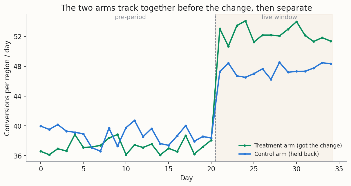
In the pre-period the two arms sit on top of each other — that overlap is the evidence the randomisation worked (the pre-period gap is just −1.6, well inside the noise). It doubles as a placebo check: run the same contrast over the pre-period, where the change has not happened yet, and only trust the live read if the arms were indistinguishable beforehand [EGGERS-2024]. At launch both arms jump: that shared jump is the season. The treatment arm then keeps climbing above the control arm, and that gap is the change.
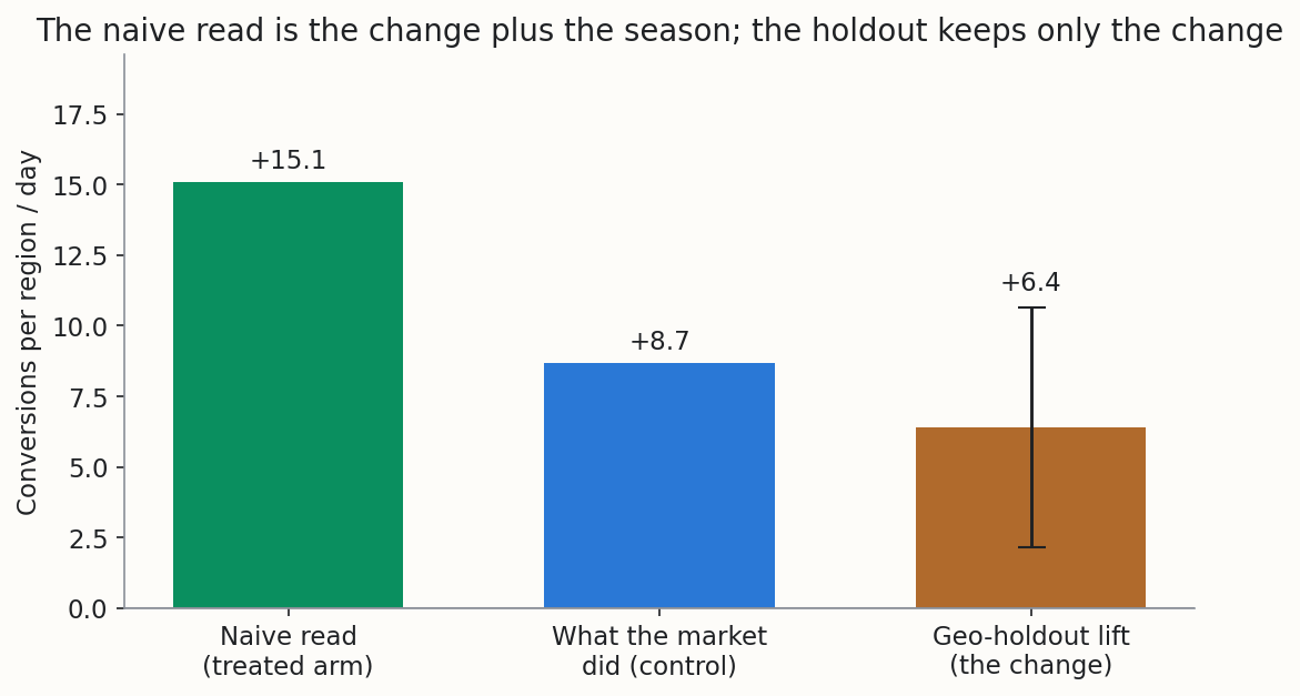
| Reading | Conv/region/day | What it is |
|---|---|---|
| Naive read (treated arm) | +15.1 | the change plus the season — what a dashboard shows |
| What the market did (control) | +8.7 | the season, revealed by the held-back regions |
| Geo-holdout lift (DiD) | +6.4 | 90% range [+2.2, +10.7] — the change alone |
The true effect we baked in was +6, so the holdout recovered it; the naive read over-credited the change by +8.7 — the entire season. Is +6.4 real, or a lucky split? The randomisation test re-shuffles which regions were “treatment” 5,000 times and asks how often a random re-split would produce a lift this big by chance:
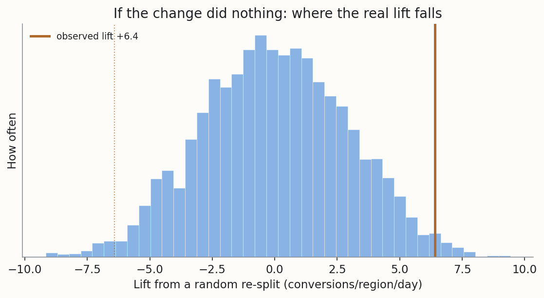
The observed lift sits out in the tail of that null distribution — a random re-split beats it only about 2.6% of the time (a p-value of 0.026). The change did something.
Run one yourself
Caveats to watch out for in this method
Every method has failure modes. Naming them is not a disclaimer; it is how you avoid making a bad call from a good-looking number.
A holdout measures the effect of this channel, in these regions, over this window — and nothing else. Last quarter’s read does not certify this quarter’s budget, and a lift measured on paid search says nothing about what a holdout on your email programme would find. A different channel or a different season needs a new test; treat a carried-over figure as a rough guide, never as proof.
When the range covers zero, the disciplined reading is that the test could not detect an effect — usually because it had too few regions or ran too short. It is not evidence the change did nothing. Reporting an underpowered null as “it doesn’t work” is how good channels get cut.
The method assumes the treated regions’ change does not reach the control regions. Two real leaks break that: audiences that straddle a market border, and platform targeting that serves outside your defined geos — Meta’s Location Expansion is the sharp example, and it must be turned off on the test campaigns. A leak makes the control arm rise too, which understates your true lift.
With only a handful of large metros that behave nothing alike, even a random split can land lopsided arms, and the simple difference is then biased. Serious implementations pair comparable regions and randomise within each pair, and trim the most extreme pairs so a couple of giant metros cannot dominate the read. When the arms cannot be balanced, the read falls back to building a synthetic control from the held-out regions — sturdier against imbalance, but no longer a pure experiment.
The control regions are deliberately left un-optimised for the window. That is a real, if temporary, price — which is why a holdout is a decision to make on purpose, for the channels big enough to be worth settling, not a thing to run on everything.
Randomising removes the confounding — the season, the competitor, the payday all cancel. It does not remove sampling noise: a different random split of the same regions would have landed a little differently, and the range is exactly that wobble. The strongest causal evidence in marketing is still a range, and anyone selling you a single certain lift number is selling you the wrong thing.
How many regions do you need?
The single most common way a geo test “fails” is that it was too small: too few regions, and the range is so wide it covers zero — which reads as “no effect” but really means “too small to tell.” The notebook holds the true effect fixed at +6 and grows the number of regions:
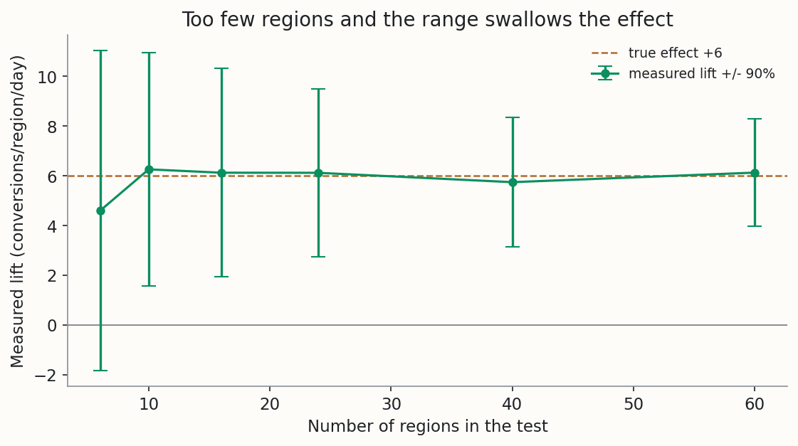
With 6 regions the lift lands around +4.6 but the range runs roughly ±6.4 — it crosses zero, and across repeated runs a test this small catches a clear result only about 38% of the time. By 40 regions the range is down near ±2.6 and a clear read comes back about 95% of the time; by 60 it is about ±2.2 and essentially always. This is why the honest first question about a geo test is not “what was the lift” but “was the test big enough to have found one.” If your range covers zero, add regions or run longer before you conclude anything.
How the industry uses it
The geo experiment is not fringe — it is the measurement the largest platforms and the serious independent shops all converge on. Google introduced the modern form (“One approach that Google has successfully employed to measure advertising effectiveness is geo experiments”[VAVER-KOEHLER-2011]) and productised it inside Google Ads, where Conversion Lift “based on geography” lets advertisers “measure the incremental conversions driven by your Google Ads campaigns” [GOOGLE-CONVERSION-LIFT]. Meta open-sourced its own version, GeoLift, “an end-to-end geo-experimental methodology based on Synthetic Control Methods used to measure the true incremental effect (Lift) of ad campaign”[GEOLIFT-META].
Independent measurement firms build their businesses on it. Recast sells a geo product that “measures the incremental conversions driven by marketing activity — separating true growth drivers from channels claiming credit for conversions they didn't actually drive”[RECAST-GEOLIFT], and treats a clean test as the yardstick everything else is calibrated against: “we believe that well-run incrementality experiments are the best estimate that a marketer has for true incrementality”[RECAST-EXPERIMENTS]. Haus describes the identical design — “markets across a specific country are randomly assigned to receive either the treatment (advertising on a specific channel) or the control (no advertising)”[HAUS-GEO] — and Measured runs “geo-matched and first-party split tests” [MEASURED-INCR]. The reads are concrete: one public retail-media case study reported “over 5.5 million impressions and a $2.41 incremental return on ad spend” from a matched-market test [MONDELEZ-ALBERTSONS].
This is the method the channel-attribution post pointed you toward: attribution finds the channels worth interrogating; a holdout is how you settle whether one of them is really driving sales.
Run it on your own data
The downloads run entirely on your machine — your data never leaves it. They take a table of daily conversions per region:
| column | meaning | example |
|---|---|---|
geo | region name or code | US-CA |
date | the day, ISO format | 2026-05-01 |
arm | treatment or control | treatment |
conversions | that region's conversions that day | 47 |
You also tell them the launch date — the first day the change went live — which splits every region's series into pre-period and live window. They validate the columns, run the same difference-in-differences, and warn you in plain words when the data is too thin to trust instead of printing a confident number. As rough rules of thumb they flag fewer than five regions per arm, a live window under seven days, arms that look unbalanced before the change, and the big one — a range that covers zero, which they label “too small to tell,” never “proven to do nothing.”
Getting your data into that shape
Most analytics exports are not a tidy region-by-day table — they are a long log of individual conversions, each stamped with a region and a date. The notebook includes a consolidate_conversions helper that does the tedious middle step: it rolls that raw log up into daily counts per region and fills in the zero-conversion days (a day with no sales is real signal, not a missing row). After that you add the arm column from the split you actually ran and set the launch date.
Where does the raw log come from? If your site sends conversions to Google Analytics 4 with the free BigQuery export on, the notebook ships a ready query that pulls one row per conversion, stamped with region and date. Swap in your conversion event and your region dimension, run it, hand the output to the consolidator, and you have the table above. Assembling and stitching that data is the part the platform automates; here we show how to do it by hand.
This part is technical — a database query and a notebook — but you do not have to do it alone. Download the give-it-to-your-AI brief and hand it to ChatGPT, Claude, or any capable assistant. It carries everything the assistant needs to walk you through getting your data and running the analysis, one step at a time, even if you have never written a line of code.
Common questions
Is a geo-holdout the same as an A/B test?
The range on my result includes zero. Did my change fail?
Do the control regions lose money?
How many regions do I need?
Can I reuse a holdout result for another channel or another quarter?
Should I drop attribution and only run holdouts?
What if my channel has no regions to split — like a CRM or email tool?
Running this on your own account
The worked example above is synthetic; the notebook runs on your data instead, and every number it gives you carries its range. If you want a hand with the method — or with the paid media underneath it — I take on freelance work, and I answer questions about anything published here.
Get in touchReferences
- [VAVER-KOEHLER-2011] Vaver, J. & Koehler, J. (2011). Measuring Ad Effectiveness Using Geo Experiments. Google Inc. https://services.google.com/fh/files/blogs/geo_experiments_final_version.pdf
- [CHEN-LONGFILS-REMY-2021] Chen, A., Longfils, M. & Remy, N. (2021). Trimmed Match Design for Randomized Paired Geo Experiments. Google, open-source library trimmed_match. https://github.com/google/trimmed_match
- [GORDON-2019] Gordon, B. R., Zettelmeyer, F., Bhargava, N. & Chapsky, D. (2019). A comparison of approaches to advertising measurement: Evidence from big field experiments at Facebook. Marketing Science 38(2), 193–225. https://doi.org/10.1287/mksc.2018.1135
- [EGGERS-2024] Eggers, A. C., Tuñón, G. & Dafoe, A. (2024). Placebo Tests for Causal Inference. American Journal of Political Science 68(3), 1106–1121. https://doi.org/10.1111/ajps.12818
- [GEOLIFT-META] Meta Open Source. GeoLift: measuring incrementality at a geo level. https://github.com/facebookincubator/GeoLift
- [GOOGLE-CONVERSION-LIFT] Google. Set up Conversion Lift based on geography. Google Ads Help (accessed 2026-07-19). https://support.google.com/google-ads/answer/14097193
- [RECAST-GEOLIFT] Recast. GeoLift by Recast (accessed 2026-07-19). https://getrecast.com/geolift-by-recast/
- [RECAST-EXPERIMENTS] Recast. How Recast incorporates experiments. Recast documentation (accessed 2026-07-19). https://docs.getrecast.com/docs/experiments
- [HAUS-GEO] Haus. Geo experiments: the fundamentals (accessed 2026-07-19). https://www.haus.io/blog/geo-experiments-the-fundamentals
- [MEASURED-INCR] Measured. Incrementality Testing (accessed 2026-07-19). https://www.measured.com/incrementality-testing/
- [MONDELEZ-ALBERTSONS] Marketing Dive. Mondelēz lifts sales as Albertsons tackles in-store retail media measurement (2026). https://www.marketingdive.com/news/mondelez-lifts-sales-albertsons-tackles-in-store-retail-media-measurement/808842/
From Stochastic Strata. We build marketing measurement that shows its working: every number carries its range, and when the data cannot answer a question, we say so — and tell you what would. The worked example here is synthetic; the method is the real thing, and you can run it on your own data with the notebook or spreadsheet above. Nothing in this post is financial advice.