Marketing mix modelling · 15 min read · Interactive · Video

How much should I spend on each channel — and where does the next euro stop paying off?

You know your cost per sale on each channel. What it can’t tell you is the question every planning cycle asks: if I had one more euro, which channel should it go to — and is any channel now so full that the next euro is close to wasted?

Andrei PopescuFounder of Stochastic Strata — eight years in media buying before turning to statistical marketing measurement.July 2026
Written against the cited papers

The short answer

Marketing mix modelling (MMM) answers the budget question by learning a diminishing-returns curve for each channel from your weekly spend and revenue, then reading the return on the next euro at the spend level you are actually running. Channels where the next euro still earns a lot have room to grow; channels where it earns little are full. Move budget from the full ones to the hungry ones and total revenue rises without spending a cent more — the one thing a per-channel average cannot give you, because the average blends the productive first euros with the wasted last ones.

In the worked example below, a per-channel cost-per-sale table makes Social look the best buy and Video the worst. The curves say the reverse: the next euro on Video returns about €2.69 (€1.93–€3.39), on Social about €0.99 (€0.86–€1.17). Move about €2,700 a week off the full channel (Social) onto the hungry one (Video), keeping total spend fixed, and weekly media-driven revenue rises about €2,061 — a 2.6% lift, near €107,000 a year, at no extra spend. The honest version is a range: the gain lands between €1,224 and €4,055 a week — €64,000 to €211,000 a year — and never crosses zero.

One caution up front: an MMM is correlational, not a controlled experiment. It is the third of three lenses — this post is the capstone that shows how attribution, a geo-holdout, and MMM triangulate to justify a budget move. The caveats to watch out for are the important part.

Watch · 8 min The capstone of the series: why attribution, a geo-holdout, and MMM together are the triangulation that justifies a budget shift — and why one channel cost-per-sale number can’t.

Watch: why you need three methods, not a glance

Prefer to read? Everything below covers the MMM half in depth — the maths, a widget to play with, and the notebook and spreadsheet to run it yourself. The video worked example is synthetic, and every on-screen number is computed. (Narration is automated for now.)

Sources cited in the video: the attribution-versus-experiment gap from Gordon et al. 2019; the saturation curve and carryover from Google’s MMM paper (Jin et al. 2017); the correlational-not-causal limit and the fit-versus-decision gap from Chan & Perry 2017; and the calibrate-against-experiments tie from Google’s Meridian and Meta’s Robyn. The full list is in the references below.

The question a per-channel average can’t answer

Picture three channels. On a spend-weighted cost-per-sale report they can look broadly similar — all "profitable," all worth keeping. But that report is an average over every euro you spent, and euros are not interchangeable. The early euros on a channel land on the steep part of its curve and work hard; the later euros land on the flat part and barely move revenue. Two channels with the same average can sit in completely different places: one still climbing, one long since flattened.

The budget decision does not live in the average. It lives in the slope at your current spend — the extra revenue the next euro would bring, which economists call the marginal return and MMM people call mROI. A channel with a high average but a flat slope is a place to stop adding; a channel with a lower average but a steep slope is a place to grow. You cannot see the slope from a spend total and a revenue total. You have to recover the whole curve.

The two shapes every channel has

Diminishing returns (saturation). Spend a little on a channel and each euro finds a fresh, receptive customer. Spend a lot and you start paying to reach people you would have reached anyway. So the curve of revenue against spend rises, then bends over, then flattens toward a ceiling. The bend is the whole story: below it you are underspending, above it you are feeding a channel that is already full.

Carryover (adstock). Advertising has an echo. Someone sees your ad this week and buys next week, so a burst of spend keeps paying out for a few weeks afterward, fading as it goes. MMM spreads each week's spend forward with a decaying weight, which matters while spend is changing; at a steady weekly budget the echo settles and the response is only the saturation curve.

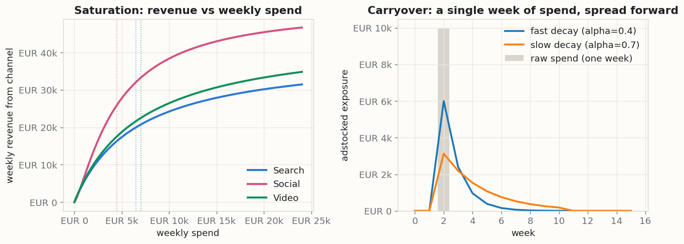
Left: a saturation curve, revenue rising then flattening as weekly spend grows. Right: carryover, a single week of spend spread forward over the following weeks and fading.

The maths, unpacked

Two transforms, applied in a specific order, then added up. None of it is more than a marketer with a spreadsheet can follow.

Saturation — the Hill curve. Each channel's revenue as a function of its (carryover-adjusted) spend x is a ceiling times an S-or-concave fraction:

contribution = β · Hill(x)Hill(x) = x^s / (x^s + ec^s)

β: the ceiling — the most weekly revenue this channel could ever add, no matter how much you pour in.
ec: the half-saturation point — the weekly spend at which the channel delivers exactly half its ceiling, because at x = ec the fraction is ½.
s: the slope, how sharply the curve bends: s ≤ 1 gives plain diminishing returns, s > 1 a gentle S that is slow to start. This is the Hill function from the foundational Google MMM paper.

Carryover — geometric adstock. Before the spend hits the curve, this week's exposure is blended with recent weeks', with the weights normalised so they sum to one:

adstock_t = ( Σ α^l x_t−l ) / ( Σ α^l )

α: the decay (between 0 and 1) — how much of last week's effect carries into this week.
l: how many weeks back you look (the standard default is eight). Because the weights sum to one, a steady spend passes through unchanged; the echo only shows up when spend moves.

The order, and the total. Carryover comes first, then saturation. Add up all the channels and a baseline (trend, season, everything non-media), and you have the model's guess at weekly revenue:

revenue_t = baseline_t + Σ_c β_c · Hill(adstock_c(x)) + noise

the slope: the number you act on is the slope of one channel's curve at your current spend — the return on the next euro. Fit the curves, read the slopes, move budget toward the steep ones.

A worked example synthetic data

The notebook invents two years — 156 weeks — of weekly data for an ecommerce brand running Search, Social, and Video. By construction the brand has over-fed one channel and starved another, and the model is told none of it. Mean revenue is about €179,000 a week, of which media drives about 44%, and the fit reports a weighted error of 2.0%. (Deliberately, it does not lead with R²: Chan & Perry showed several models fitting the same data within a few percent yet disagreeing by up to 50% on what to do about it.)

The brand spends €26,096 a week — about €1.36M a year, split€13,404 Social (51%), €8,899 Search (34%), €3,793 Video (15%). Those totals matter for reading everything below: the reallocation this post arrives at moves€2,681 — a tenth of the whole budget, and a fifth of Social’s own spend — so it is a real reweighting of a mid-sized account, not a rounding adjustment on a giant one.

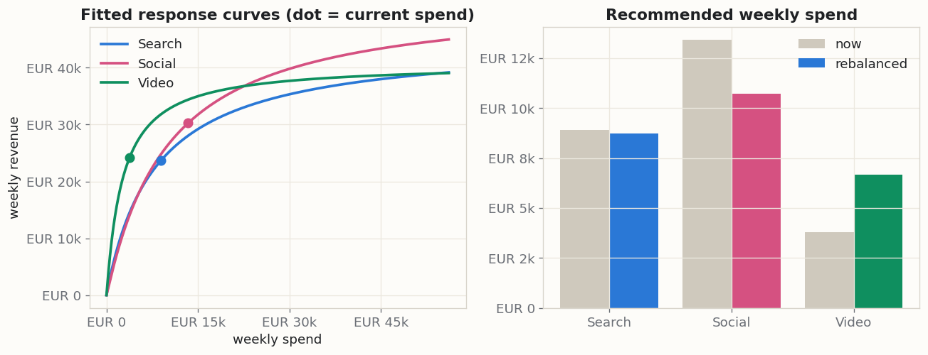
Left: fitted response curves for Search, Social and Video, each with a dot at its current spend. Right: current versus recommended weekly spend per channel — Social down, Video up.

Here is what the model reads off the fitted curves — the return on the next euro at each channel's current spend, with a 90% range from resampling the data many times:

Channel	Spending now	Next euro returns	90% range
Video	€3,793/wk	€2.69	€1.93 – €3.39
Search	€8,899/wk	€1.24	€1.03 – €1.50
Social	€13,404/wk	€0.99	€0.86 – €1.17

The gap is the recommendation. Video is underfed — every extra euro is still returning close to three, so it has room. Social is full — it has the most spend and the lowest next-euro return, so its marginal euro is nearly breaking even. So the model moves budget from the full channel to the hungry one, keeping total spend fixed: take €2,681 a week off Social, put €2,861 onto Video (the small remainder comes off Search), and weekly media-driven revenue rises by about €2,061 — a 2.6% lift, about €107,000 a year, at no extra spend. The honest version of that number is a range: 90% of the resampled fits land the gain between €1,224 and €4,055 a week — carried across a year, €64,000 to €211,000. It never crosses zero, so the direction is safe even though the exact size is not.

Read the annual figures with two things in mind. They are the weekly result multiplied by fifty-two, which assumes the effect holds steady all year — no seasonality, no saturation shifting as Video is fed, no competitor response; the weekly number is the modelled quantity and the annual one is an extrapolation of it. And the whole worked example runs on synthetic data, so this is a modelled result demonstrating a method, not a measured outcome from a real account.

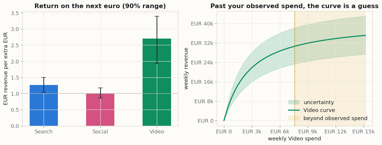
Left: the return on the next euro for each channel with its 90% range. Right: past the observed spend range, the Video curve fans out into a widening band — the model is extrapolating.

One caveat is baked into the recommendation itself. The suggested Video spend sits right at the top of what this brand has actually run. Push much further and the model is extrapolating, and the honest range fans out fast — which is the perfect segue to the ways MMM misleads you.

Interactive Drag each channel's weekly spend and watch the return on the next euro — and the reallocation gain — change in real time. This runs the same saturation maths in your browser; nothing leaves the page.

Play with the budget

Caveats to watch out for in this method

Every method has failure modes. Naming them is not a disclaimer; it is how you avoid making a bad call from a good-looking number.

It is correlational, not causal.

An MMM reads history and finds patterns; it cannot prove a channel caused the sales. In Google’s own words, "MMMs are regression models based on a limited amount of aggregated observational data and such models produce correlational, not causal results." Use it to decide what to test, then confirm the big moves with an experiment — a geo holdout is the natural partner.

Spend that rises with hidden demand fools it.

If you spend more exactly when demand is already high — the season, a product launch, a trend — the model can hand the credit to the ads for sales the demand would have produced anyway. This "selection bias" is, in Google’s own assessment, the single biggest threat to an MMM’s honesty, and no amount of curve-fitting removes it.

Targeted channels look better than they are.

Retargeting and brand search point ads at people who already want the product. The model sees those channels sitting next to conversions and credits them, when much of that would have converted regardless. Read a suspiciously high return on a bottom-of-funnel channel with that in mind — and settle it with a holdout.

Channels that moved together can’t be told apart.

The model can only separate two channels if their spend varied independently. If you always scaled two channels up and down together, their histories are nearly identical and the fit splits the credit arbitrarily — their combined effect is solid, the split between them is not. In the notebook, forcing two channels into lockstep drives their correlation to 0.95 and the warning fires. The fix is to deliberately vary their budgets apart for a few weeks, or report them as one bucket.

Past your observed spend, the curve is a guess.

The saturation shape is learned from the spend range you have actually run. Ask "what if I double it?" and the model is extrapolating into territory it has never seen — and several curves that fit your history equally well fan out to very different answers out there. Trust a recommendation near where you already spend; treat one that pushes far beyond it as a hypothesis to step toward gradually, not a promise.

A great fit is not a great answer.

Because sales vary far more than spend does, many models fit the data well yet disagree sharply on the budget advice — in Chan & Perry’s example, models within a few percent of each other on fit differed by up to 50% on predicted sales. This is why every number here is a range, and why the responsible move is to disclose how much of the answer came from the data versus the modeller’s assumptions.

Why you need three methods, not a glance

Start where most budget decisions start: a per-channel cost-per-sale table. On the synthetic advertiser in the video, that table makes Social look the best buy — the lowest cost per sale, near €22 — and Video the worst, near €40. The obvious move is to feed Social and cut Video. It is exactly backwards, and the reason is that one cost-per-sale number is quietly answering three different questions at once: who earned the sale, whether the channel caused it, and whether the next euro still works. Blur the three together and the number can point the wrong way. Separating them takes three different methods — the three posts in this series.

Attribution fixes the credit. The Markov removal effect re-credits across the whole journey: Video opens journeys it rarely closes, so its credit climbs from a tenth to about a third, while Social — a closer — falls from two-thirds. Put that back into cost-per-sale and the table turns over: Video becomes the cheapest, Social the dearest. But attribution reads history; it cannot prove Video caused a sale. A geo-holdout fixes the cause. Turn each channel off in test regions and measure the drop: Video's incremental return clears break-even comfortably; Social's straddles it — much of what Social "converts" is demand that would have arrived anyway. But a holdout settles one channel at a time, at a cost, and gives no curve. MMM fixes the saturation. It reads the whole budget's response curves and hands you the reallocation above — Video underfed, Social full — but it is correlational, so it can be fooled by hidden demand.

That is the point of triangulation: three independent methods, each strongest exactly where the last is blind — credit, cause, saturation. They use different data and different maths, so when all three point the same way (feed Video, trim Social), the agreement is far stronger evidence than any one of them alone, and incomparably stronger than eyeballing a single number that carries all three weaknesses at once. It is the same move as a holdout cancelling the season by subtracting a control group — one level up, cancelling method bias. When the three disagree, the disagreement is itself the finding: we report the split, trust the experiment on cause, and name what would settle it. The best versions close the loop — Google's Meridian is built to "set custom ROI priors using past experiments," feeding a holdout's causal lift into the model as its starting point. No single number here is the truth; the confidence comes from independent methods agreeing, and from stating the range when they do not.

How the industry uses it

MMM is not a niche technique — it is the method the biggest platforms have each open-sourced and put their name to. Google ships Meridian, "an open-source MMM built by Google" designed "to estimate the true causal impact of your marketing" [MERIDIAN]. Meta ships Robyn, "an experimental, AI/ML-powered and open sourced Marketing Mix Modeling (MMM) package from Meta Marketing Science" [ROBYN-DOCS]. And the open-source PyMC-Marketing library offers a Bayesian media-mix model using exactly the pieces in this post — geometric adstock and a saturation transform [PYMC-MMM]. The maths here is the maths they run.

Its resurgence is not fashion — it is privacy. Because MMM works from aggregate weekly numbers rather than individual tracking, it survives the collapse of cookies and device IDs that broke click-based measurement: one vendor notes it "relies on aggregated spend and outcome data (not user-level tracking)" and so is "largely unaffected by signal loss from cookie deprecation, iOS privacy updates, or walled garden policies" [MMM-PRIVACY-NORTHBEAM]; another that it "does not depend on browser policies or platform changes" [MMM-PRIVACY-MEASURED]. That is why a technique from the television era is back at the centre of modern stacks, alongside vendors like Analytic Partners [ANALYTICPARTNERS-DEF].

The reads are concrete: Meta's own Robyn case studies include one titled "How Resident Increased Revenue 20% by Adopting Facebook's Open-Source MMM Solution" [RESIDENT-CASE] — a reported case for a different advertiser, not a promise about yours. And the serious versions close the honesty gap the same way we recommend: Google's Meridian is built to "set custom ROI priors using past experiments" [MERIDIAN] — calibrating the correlational model against real incrementality tests. That is the same move as pairing an MMM with a geo holdout: the model narrows the field and sizes the curves; an experiment confirms the big bets.

Run it on your own data

Every download runs entirely on your machine — your data never leaves it. They take one weekly panel: a row per week, with the revenue that week and one spend column per channel.

column	meaning	example
`week`	Monday of the week	`2024-01-01`
`revenue`	total revenue that week	`184320`
`spend_<channel>`	one column per channel	`spend_Search` = `9100`
`control_<name>` (optional)	anything else that moves sales	`control_promo` = `1`

The notebook refuses to give a confident answer it cannot support: fewer than 52 weeks and it stops (you need a full year of seasonality first); thin data and it labels every number an estimate and tells you to read the ranges; two channels that moved together and it warns you it cannot split them.

Notebook · PythonThe full method, executableFits the saturation-and-carryover curves from your weekly panel, reads each channel's next-euro return with a 90% range, proposes the rebalance, and regenerates every figure here. Refuses under 52 weeks; warns on thin data and on channels that moved together.Spreadsheet · ExcelThe reallocation, in live cellsA simplified three-sheet workbook: the article's fitted curves as live formulas, a reallocation playground (edit the split, watch the weekly gain), and a your-data sheet that ranks next-euro returns and flags a channel pushed past its observed spend. Every cell is a formula.PDF · for your AIGive it to your assistantA hand-to-your-AI brief: give it to ChatGPT or Claude and it walks you through assembling your weekly spend-and-revenue table and running the notebook, one step at a time — with every caveat stated up front — no code experience needed.

Getting your data into that shape

Most exports are daily, not the weekly table the model needs, so the notebook ships a daily_to_weekly consolidator that rolls a daily spend log and a daily revenue series up into the weekly panel automatically. The raw material is a weekly spend figure per channel (from Google Ads and Meta) and weekly revenue (from GA4 or your shop) — the same numbers your finance export already has. Because MMM works from those aggregates alone, it needs no cookies, device IDs, or user-level tracking.

The one real judgement call is the channel definition — mapping your campaigns into a handful of channels — because spend lives under campaign names in each platform, not tidy buckets. And use the system that sees all your sales for revenue (GA4 or your shop), not a single ad platform's reported revenue, which double-counts across platforms and misses offline sales.

This part touches a spreadsheet or a light script — but you do not have to do it alone. Download the give-it-to-your-AI brief and hand it to ChatGPT, Claude, or any capable assistant. It carries everything the assistant needs to pull your data, shape it, and run the notebook, one step at a time, even if you have never written a line of code.

Common questions

Is MMM the same as attribution?

No — they answer different questions. Attribution (last-click, or the Markov removal effect) reads individual customer journeys to see which channels show up on the paths that convert. MMM ignores journeys entirely and works from weekly totals, learning how much revenue each channel’s spend produces and where it saturates. Attribution is a within-week, journey-level lens; MMM is a monthly, budget-level one. Serious teams run both and triangulate.

How much data do I need?

At least a full year — 52 weeks — so the model can see a whole cycle of seasonality; below that the notebook refuses to answer. Two to three years is better. The real constraint is data points per thing you are estimating: with only a couple of years of national weekly data, an MMM is stretched thin and its ranges will be wide. Wide ranges are the model being honest, not broken.

Does it need cookies or user tracking?

No, and that is much of why it is resurging. MMM runs on aggregate weekly spend and revenue — numbers you already have in a finance export — so it is untouched by cookie deprecation, iOS tracking prompts, and consent walls. It is the privacy-durable half of a modern measurement stack.

Can I trust the exact euro figures?

Trust the direction more than the decimals. The reliable output is the ranking of next-euro returns and the rebalance direction — feed the hungry channel, trim the full one. The precise gain is a range, and the individual curve shapes are the least certain part of the fit. Anyone reporting an MMM result as a single confident number is overselling it.

My model says to pour money into one channel. Should I?

Only if the recommended spend is near where you have actually spent before. If it pushes far past your observed range, the model is guessing the curve out there — step the budget up gradually so each increase gives it real data at the new level, and confirm a big move with an experiment first.

Should I build this myself or buy a tool?

The method is open — Google’s Meridian, Meta’s Robyn, and PyMC-Marketing are all free and capable, and the notebook here is a working miniature. What a platform adds is not the model but everything around it: assembling clean weekly data, keeping it current, catching the caveats above automatically, and calibrating the curves against real experiments. The maths is the easy part.

Running this on your own account

The worked example above is synthetic; the notebook runs on your data instead, and every number it gives you carries its range. If you want a hand with the method — or with the paid media underneath it — I take on freelance work, and I answer questions about anything published here.

Get in touch

References

[JIN-2017] Jin, Y., Wang, Y., Sun, Y., Chan, D. & Koehler, J. (2017). Bayesian Methods for Media Mix Modeling with Carryover and Shape Effects. Google Inc. https://research.google/pubs/bayesian-methods-for-media-mix-modeling-with-carryover-and-shape-effects/
[CHAN-2017] Chan, D. & Perry, M. (2017). Challenges and Opportunities in Media Mix Modeling. Google Inc. https://research.google/pubs/challenges-and-opportunities-in-media-mix-modeling/
[MERIDIAN] Google for Developers. Meridian: Introduction (Meridian documentation). Google, 2025 (accessed 2026-07-23). Includes "Set custom ROI priors using past experiments". https://developers.google.com/meridian/docs/basics/meridian-introduction
[ROBYN-DOCS] Meta Marketing Science. Welcome to Robyn (Robyn documentation). Meta (accessed 2026-07-23). https://facebookexperimental.github.io/Robyn/docs/welcome/
[RESIDENT-CASE] Meta Marketing Science. Case Studies — "How Resident Increased Revenue 20% by Adopting Facebook’s Open-Source MMM Solution" (Robyn documentation). Meta (accessed 2026-07-23). https://facebookexperimental.github.io/Robyn/docs/case-studies/
[PYMC-MMM] PyMC-Marketing. MMM Example Notebook (official documentation). PyMC Labs (accessed 2026-07-23). https://www.pymc-marketing.io/en/stable/notebooks/mmm/mmm_example.html
[GORDON-2019] Gordon, B. R., Zettelmeyer, F., Bhargava, N. & Chapsky, D. (2019). A comparison of approaches to advertising measurement: Evidence from big field experiments at Facebook. Marketing Science 38(2), 193–225. https://doi.org/10.1287/mksc.2018.1135
[MMM-PRIVACY-NORTHBEAM] Northbeam. What is Media Mix Modeling (MMM)? (blog) (accessed 2026-07-23). https://www.northbeam.io/blog/media-mix-modeling-mmm-guide
[MMM-PRIVACY-MEASURED] Measured. Eight (8) Benefits of Media Mix Modeling (MMM) for Modern Marketing (FAQ) (accessed 2026-07-23). https://www.measured.com/faq/eight-8-benefits-of-media-mix-modeling-mmm/
[ANALYTICPARTNERS-DEF] Analytic Partners. Marketing Mix Modeling (solutions page) (accessed 2026-07-23). https://analyticpartners.com/solutions/marketing-mix-modeling/

From Stochastic Strata. We build marketing measurement that shows its working: every number carries its range, and when the data cannot answer a question, we say so — and tell you what would. The worked example here is synthetic; the method is the real thing, and you can run it on your own data with the notebook or spreadsheet above. Nothing in this post is financial advice.